For want of a nail the shoe was lost.
For want of a shoe the horse was lost.
For want of a horse the rider was lost.
For want of a rider the message was lost.
For want of a message the battle was lost.
For want of a battle the kingdom was lost.
And all for the want of a horseshoe nail.
Was the kingdom lost due to random chance? Or was it the inevitable outcome resulting from sensitive dependence on initial conditions? Does the difference even matter? Here is a blog post about Chaos and Randomness with Julia code.
Preliminaries
Consider a real vector space $X$ and a function $f: X \to X$ on that space. If we repeatedly apply $f$ to a starting vector $x_1$, we get a sequence of vectors known as an orbit $x_1, x_2, ... ,f^n(x_1)$.
For example, the logistic map is defined as
function logistic_map(r, x)
r*x*(1-x)
end
Here is a plot of successive applications of the logistic map for r=3.5. We can see that the system constantly oscillates between two values, ~0.495 and ~0.812.

Definition of Chaos
There is surprisingly no universally accepted mathematical definition of Chaos. For now we will present a commonly used characterization by Devaney:

We can describe an orbit $x_1, x_2, ... ,f^n(x_1)$ as *chaotic* if:
- The orbit is not asymptotically periodic, meaning that it never starts repeating, nor does it approach an orbit that repeats (e.g. $a, b, c, a, b, c, a, b, c...$).
- The maximum Lyapunov exponent $\lambda$ is greater than 0. This means that if you place another trajectory starting near this orbit, it will diverge at a rate $e^\lambda$. A positive $\lambda$ implies that two trajectories will diverge exponentially quickly away from each other. If $\lambda<0$, then the distance between trajectories would shrink exponentially quickly. This is the basic definition of "Sensitive Dependence to Initial Conditions (SDIC)", also colloquially understood as the "butterfly effect".
Note that (1) intuitively follows from (2), because the Lyapunov exponent of an orbit that approaches a periodic orbit would be $<0$, which contradicts the SDIC condition.
We can also define the map $f$ itself to be chaotic if there exists an invariant (trajectories cannot leave) subset $\tilde{X} \subset X$, where the following three conditions hold:


- Sensitivity to Initial Conditions, as mentioned before.
- Topological mixing (every point in orbits in $\tilde{X}$ approaches any other point in $\tilde{X}$).
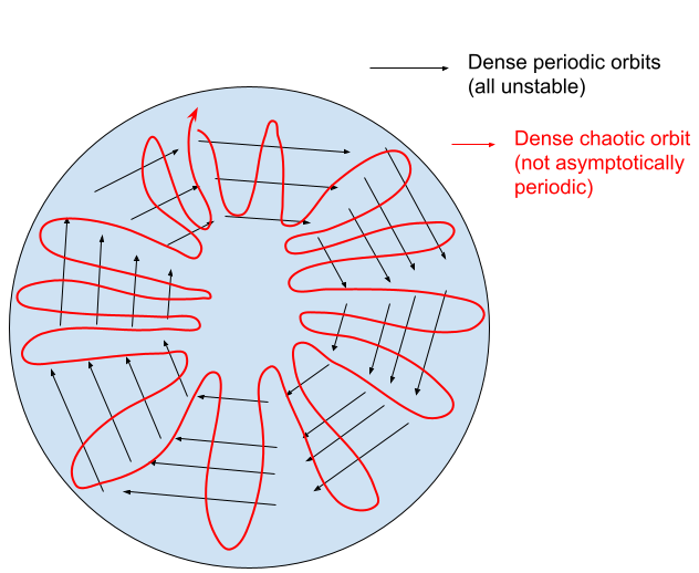
- Dense periodic orbits (every point in $\tilde{X}$ is arbitrarily close to a periodic orbit). At first, this is a bit of a head-scratcher given that we previously defined an orbit to be chaotic if it *didn't* approach a periodic orbit. The way to reconcile this is to think about the subspace $\tilde{X}$ being densely covered by periodic orbits, but they are all unstable so the chaotic orbits get bounced around $\tilde{X}$ for all eternity, never settling into an attractor but also unable to escape $\tilde{X}$.
Note that SDIC actually follows from the second two conditions. If these unstable periodic orbits cover the set $\tilde{X}$ densely and orbits also cover the set densely while not approaching the periodic ones, then intuitively the only way for this to happen is if all periodic orbits are unstable (SDIC).
These are by no means the only way to define chaos. The DynamicalSystems.jl package has an excellent documentation on several computationally tractable definitions of chaos.
Chaos in the Logistic Family
Incidentally, the logistic map exhibits chaos for most of the values of r from values 3.56995 to 4.0. We can generate the bifurcation diagram quickly thanks to Julia's de-vectorized way of numeric programming.
rs = [2.8:0.01:3.3; 3.3:0.001:4.0]
x0s = 0.1:0.1:0.6
N = 2000 # orbit length
x = zeros(length(rs), length(x0s), N)
# for each starting condtion (across rows)
for k = 1:length(rs)
# initialize starting condition
x[k, :, 1] = x0s
for i = 1:length(x0s)
for j = 1:N-1
x[k, i, j+1] = logistic_map((r=rs[k] , x=x[k, i, j])...)
end
end
end
plot(rs, x[:, :, end], markersize=2, seriestype = :scatter, title = "Bifurcation Diagram (Logistic Map)")
We can see how starting values y1=0.1, y2=0.2, ...y6=0.6 all converge to the same value, oscillate between two values, then start to bifurcate repeatedly until chaos emerges as we increase r.

Spatial Precision Error + Chaos = Randomness
What happens to our understanding of the dynamics of a chaotic system when we can only know the orbit values with some finite precision? For instance, x=0.76399 or x=0.7641 but we only observe x=0.764 in either case.
We can generate 1000 starting conditions that are identical up to our measurement precision, and observe the histogram of where the system ends up after n=1000 iterations of the logistic map.

Let's pretend this is a probabilistic system and ask the question: what are the conditional distributions of $p(x_n|x_0)$, where $n=1000$, for different levels of measurement precision?
At less than $O(10^{-8})$ precision, we start to observe the entropy of the state evolution rapidly increasing. Even though we know that the underlying dynamics are deterministic, measurement uncertainty (a form of aleotoric uncertainty) can expand exponentially quickly due to SDIC. This results in $p(x_n|x_0)$ appearing to be a complicated probability distribution, even generating "long tails".
I find it interesting that the "multi-modal, probabilistic" nature of $p(x_n|x_0)$ vanishes to a simple uni-modal distribution when measurement is sufficiently high to mitigate chaotic effects for $n=1000$. In machine learning we concern ourselves with learning fairly rich probability distributions, even going as far as to learn transformations of simple distributions into more complicated ones.
But what if we are being over-zealous with using powerful function approximators to model $p(x_n|x_0)$? For cases like the above, we are discarding the inductive bias that $p(x_n|x_0)$ arises from a simple source of noise (uniform measurement error) coupled with a chaotic "noise amplifier". Classical chaos on top of measurement error will indeed produce Indeterminism, but does that mean we can get away with treating $p(x_n|x_0)$ as purely random?
I suspect the apparent complexity of many "rich" probability distributions we encounter in the wild are more often than not just chaos+measurement error (e.g. weather). If so, how can we leverage that knowledge to build more useful statistical learning algorithms and draw inferences?
We already know that chaos and randomness are nearly equivalent from the perspective of computational distinguishability. Did you know that you can use chaos to send secret messages? This is done by having Alice and Bob synchronize a chaotic system $x$ with the same initial state $x_0$, and then Alice sends a message $0.001*signal + x$. Bob merely evolves the chaotic system $x$ on his own and subtracts it to recover the signal. Chaos has also been used to design pseudo-random number generators.
No comments:
Post a Comment
Comments will be reviewed by administrator (to filter for spam and irrelevant content).