In this blog post, we abandoned all pretense of theoretical rigor and used pixel values from natural images as learning rate schedules.

The learning rate schedule is an important hyperparameter to choose when training neural nets. Set the learning rate too high, and the loss function may fail to converge. Set the learning rate too low, and the model may take a long time to train, or even worse, overfit.
The optimal learning rate is commensurate with the scale of the smoothness of the gradient of the loss function (or in fancy words, the “Lipschitz constant” of a function). The smoother the function, the larger the learning rate we are allowed to take without the optimization “blowing up”.
What is the right learning rate schedule? Exponential decay? Linear decay? Piecewise constant? Ramp up then down? Cyclic? Warm restarts? How big should the batch size be? How does this all relate to generalization (what ML researchers care about)?
The optimal learning rate is commensurate with the scale of the smoothness of the gradient of the loss function (or in fancy words, the “Lipschitz constant” of a function). The smoother the function, the larger the learning rate we are allowed to take without the optimization “blowing up”.
Tragically, in the non-convex, messy world of deep neural networks, all theoretical convergence guarantees are off. Often those guarantees rely on a restrictive set of assumptions, and then the theory-practice gap is written off by showing that it also “empirically works well” at training neural nets.
Fortunately, the research community has spent thousands of GPU years establishing empirical best practices for the learning rate:

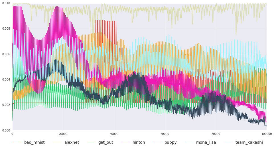
Given that theoretically-motivated learning rate scheduling is really hard, we ask, "why not use a learning rate schedule which is at least aesthetically pleasing?" Specifically, we scan across a nice-looking image one pixel at a time, and use the pixel intensities as our learning rate schedule.
We begin with a few observations:
- Optimization of non-convex objectives seem to benefit from injecting “temporally correlated noise” into the parameters we are trying to optimize. Accelerated stochastic gradient descent methods also exploit temporally correlated gradient directions via momentum. Stretching this analogy a bit, we note that in reinforcement learning, auto-correlated noise seems to be beneficial for state-dependent exploration (1, 2, 3, 4).
- Several recent papers (5, 6, 7) suggest that waving learning rates up and down are good for deep learning.
- Pixel values from natural images have both of the above properties. When reshaped into a 1-D signal, an image waves up and down in a random manner, sort of like Brownian motion. Natural images also tend to be lit from above, which lends to a decaying signal as the image gets darker on the bottom.
- baseline: The default learning rate schedules provided by the github repository.
- fixed: 3e-4 with Momentum Optimizer.
- andrej: 3e-4, with Adam Optimizer
- cyclic: Cyclic learning rates according to the following code snippet:
base_lr = 1e-5
max_lr = 1e-2
step_size = 1000
step = tf.cast(global_step, tf.float32)
cycle = tf.floor(1+step/(2*step_size))
x = tf.abs(step/step_size - 2*cycle + 1)
learning_rate = base_lr + (max_lr-base_lr)*tf.maximum(0., (1.-x))
max_lr = 1e-2
im = Image.open(path_to_file)
num_steps = _NUM_IMAGES['train']*FLAGS.train_epochs/FLAGS.batch_size
w, h = im.size
f = np.sqrt(w*h*3/num_steps)
im = im.resize((int(float(w)/f), int(float(h)/f)))
im = np.array(im).flatten().astype(np.float32)/255
im_t = tf.constant(im)
step = tf.minimum(global_step, im.size-1)
pixel_value = im_t[step]
learning_rate = base_lr + (max_lr - base_lr) * pixel_value
We chose some very aesthetically pleasing images for our experiments.
Which one gives the best learning rate?

max_lr = 1e-2
step_size = 1000
step = tf.cast(global_step, tf.float32)
cycle = tf.floor(1+step/(2*step_size))
x = tf.abs(step/step_size - 2*cycle + 1)
learning_rate = base_lr + (max_lr-base_lr)*tf.maximum(0., (1.-x))
- image-based learning rates using the following code:
max_lr = 1e-2
im = Image.open(path_to_file)
num_steps = _NUM_IMAGES['train']*FLAGS.train_epochs/FLAGS.batch_size
w, h = im.size
f = np.sqrt(w*h*3/num_steps)
im = im.resize((int(float(w)/f), int(float(h)/f)))
im = np.array(im).flatten().astype(np.float32)/255
im_t = tf.constant(im)
step = tf.minimum(global_step, im.size-1)
pixel_value = im_t[step]
learning_rate = base_lr + (max_lr - base_lr) * pixel_value
Candidate Images
We chose some very aesthetically pleasing images for our experiments.
 |
| alexnet.jpg |
 |
| bad_mnist.jpg (MNIST training image labeled as a 4) |
 |
| get_out.jpg |
 |
| hinton.jpg |
 |
| mona_lisa.jpg |
 |
| team_kakashi.jpg |
 |
| puppy.jpg |
Which one gives the best learning rate?
Results
Here are the top-1 accuracies on the CIFAR-10 validation set. All learning rate schedules are trained with the Momentum Optimizer (except andrej, where we use Adam).
The default learning rate schedules provided by the github repo are quite strong, beating all of our alternative learning rate schedules.
The Mona Lisa and puppy images turns out to be a pretty good schedules, even better than cyclic learning rates and Andrej Karpathy’s favorite 3e-4 with Adam. The "bad MNIST" digit appears to be a pretty dank learning rate schedule too, just edging out Geoff’s portrait (you’ll have to imagine the error bars on your own). All learning rates perform about equally well on MNIST.
The fixed learning rate of 3e-4 is quite bad (unless one uses the Adam optimizer). Our experiments suggest that maybe pretty much any learning rate schedule can outperform a fixed one, so if ever you see or think about writing a paper with a constant learning rate, just use literally any schedule instead. Even a silly one. And then cite this blog post.
Future Work
- Does there exist a “divine” natural image whose learning rate schedule results in low test error among a wide range of deep learning tasks?
- It would also be interesting to see if all images of puppies produce good learning rate schedules. We think it is very likely, since all puppers are good boys.
- Stay tuned for “Aesthetically Pleasing Parameter Noise for Reinforcement Learning” and “Aesthetically Pleasing Random Seeds for Neural Architecture Search”.