Chaos and Randomness

For want of a nail the shoe was lost.

For want of a shoe the horse was lost.

For want of a horse the rider was lost.

For want of a rider the message was lost.

For want of a message the battle was lost.

For want of a battle the kingdom was lost.

And all for the want of a horseshoe nail.

- For Want of a Nail

Was the kingdom lost due to random chance? Or was it the inevitable outcome resulting from sensitive dependence on initial conditions? Does the difference even matter? Here is a blog post about Chaos and Randomness with Julia code.

Preliminaries

Consider a real vector space $X$ and a function $f: X \to X$ on that space. If we repeatedly apply $f$ to a starting vector $x_1$, we get a sequence of vectors known as an orbit $x_1, x_2, ... ,f^n(x_1)$. 

For example, the logistic map is defined as 

function logistic_map(r, x)

   r*x*(1-x) 

end

Here is a plot of successive applications of the logistic map for r=3.5. We can see that the system constantly oscillates between two values, ~0.495 and ~0.812. 

Definition of Chaos

There is surprisingly no universally accepted mathematical definition of Chaos. For now we will present a commonly used characterization by Devaney: 

We can describe an orbit $x_1, x_2, ... ,f^n(x_1)$ as *chaotic* if:

1. The orbit is not asymptotically periodic, meaning that it never starts repeating, nor does it approach an orbit that repeats (e.g. $a, b, c, a, b, c, a, b, c...$).
2. The maximum Lyapunov exponent $\lambda$ is greater than 0. This means that if you place another trajectory starting near this orbit, it will diverge at a rate $e^\lambda$. A positive $\lambda$ implies that two trajectories will diverge exponentially quickly away from each other. If $\lambda<0$, then the distance between trajectories would shrink exponentially quickly. This is the basic definition of "Sensitive Dependence to Initial Conditions (SDIC)", also colloquially understood as the "butterfly effect".

Note that (1) intuitively follows from (2), because the Lyapunov exponent of an orbit that approaches a periodic orbit would be $<0$, which contradicts the SDIC condition.

We can also define the map $f$ itself to be chaotic if there exists an invariant (trajectories cannot leave) subset $\tilde{X} \subset X$, where the following three conditions hold:

1. Sensitivity to Initial Conditions, as mentioned before.
2. Topological mixing (every point in orbits in $\tilde{X}$ approaches any other point in $\tilde{X}$).
3. Dense periodic orbits (every point in $\tilde{X}$ is arbitrarily close to a periodic orbit). At first, this is a bit of a head-scratcher given that we previously defined an orbit to be chaotic if it *didn't* approach a periodic orbit. The way to reconcile this is to think about the subspace $\tilde{X}$ being densely covered by periodic orbits, but they are all unstable so the chaotic orbits get bounced around $\tilde{X}$ for all eternity, never settling into an attractor but also unable to escape $\tilde{X}$.

Note that SDIC actually follows from the second two conditions. If these unstable periodic orbits cover the set $\tilde{X}$ densely and orbits also cover the set densely while not approaching the periodic ones, then intuitively the only way for this to happen is if all periodic orbits are unstable (SDIC).

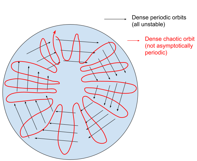
These are by no means the only way to define chaos. The DynamicalSystems.jl package has an excellent documentation on several computationally tractable definitions of chaos.

Chaos in the Logistic Family

Incidentally, the logistic map exhibits chaos for most of the values of r from values 3.56995 to 4.0. We can generate the bifurcation diagram quickly thanks to Julia's de-vectorized way of numeric programming.

rs = [2.8:0.01:3.3; 3.3:0.001:4.0]

x0s = 0.1:0.1:0.6

N = 2000 # orbit length

x = zeros(length(rs), length(x0s), N)

# for each starting condtion (across rows)

for k = 1:length(rs)

    # initialize starting condition

    x[k, :, 1] = x0s

    for i = 1:length(x0s)

       for j = 1:N-1

            x[k, i, j+1] = logistic_map((r=rs[k] , x=x[k, i, j])...)

       end

    end

end

plot(rs, x[:, :, end], markersize=2, seriestype = :scatter, title = "Bifurcation Diagram (Logistic Map)")

We can see how starting values y1=0.1, y2=0.2, ...y6=0.6 all converge to the same value, oscillate between two values, then start to bifurcate repeatedly until chaos emerges as we increase r.

Spatial Precision Error + Chaos = Randomness

What happens to our understanding of the dynamics of a chaotic system when we can only know the orbit values with some finite precision? For instance,  x=0.76399 or x=0.7641 but we only observe x=0.764 in either case.

We can generate 1000 starting conditions that are identical up to our measurement precision, and observe the histogram of where the system ends up after n=1000 iterations of the logistic map.

Let's pretend this is a probabilistic system and ask the question: what are the conditional distributions of $p(x_n|x_0)$, where $n=1000$, for different levels of measurement precision?

At less than $O(10^{-8})$ precision, we start to observe the entropy of the state evolution rapidly increasing. Even though we know that the underlying dynamics are deterministic, measurement uncertainty (a form of aleotoric uncertainty) can expand exponentially quickly due to SDIC. This results in $p(x_n|x_0)$ appearing to be a complicated probability distribution, even generating "long tails".

I find it interesting that the "multi-modal, probabilistic" nature of $p(x_n|x_0)$ vanishes to a simple uni-modal distribution when measurement is sufficiently high to mitigate chaotic effects for $n=1000$. In machine learning we concern ourselves with learning fairly rich probability distributions, even going as far as to learn transformations of simple distributions into more complicated ones. 

But what if we are being over-zealous with using powerful function approximators to model $p(x_n|x_0)$? For cases like the above, we are discarding the inductive bias that $p(x_n|x_0)$ arises from a simple source of noise (uniform measurement error) coupled with a chaotic "noise amplifier". Classical chaos on top of measurement error will indeed produce Indeterminism, but does that mean we can get away with treating $p(x_n|x_0)$ as purely random?

I suspect the apparent complexity of many "rich" probability distributions we encounter in the wild are more often than not just chaos+measurement error (e.g. weather). If so, how can we leverage that knowledge to build more useful statistical learning algorithms and draw inferences?

We already know that chaos and randomness are nearly equivalent from the perspective of computational distinguishability. Did you know that you can use chaos to send secret messages? This is done by having Alice and Bob synchronize a chaotic system $x$ with the same initial state $x_0$, and then Alice sends a message $0.001*signal + x$. Bob merely evolves the chaotic system $x$ on his own and subtracts it to recover the signal. Chaos has also been used to design pseudo-random number generators. 

Uncertainty: a Tutorial

A PDF version of this post can be found here.
Chinese translation by Xiaoyi Yin

Notions of uncertainty are tossed around in conversations around AI safety, risk management, portfolio optimization, scientific measurement, and insurance. Here are a few examples of colloquial use:

• "We want machine learning models to know what they don't know.''
• "An AI responsible for diagnosing patients and prescribing treatments should tell us how confident it is about its recommendations.''
• "Significant figures in scientific calculations represent uncertainty in measurements.''
• "We want autonomous agents to explore areas where they are uncertain (about rewards or predictions) so that they may discover sparse rewards.''
• "In portfolio optimization, we want to maximize returns while limiting risk.''
• "US equity markets finished disappointingly in 2018 due to increased geopolitical uncertainty.''

What exactly then, is uncertainty? 

Uncertainty measures reflect the amount of dispersion of a random variable. In other words, it is a scalar measure of how "random" a random variable is. In finance, it is often referred to as risk.

There is no single formula for uncertainty because there are many different ways to measure dispersion: standard deviation, variance, value-at-risk (VaR), and entropy are all appropriate measures. However, it's important to keep in mind that a single scalar number cannot paint a full picture of "randomness'', as that would require communicating the entire random variable itself! 

Nonetheless, it is helpful to collapse randomness down to a single number for the purposes of optimization and comparison. The important thing to remember is that "more uncertainty'' is usually regarded as "less good'' (except in simulated RL experiments).

Types of Uncertainty

Statistical machine learning concerns itself with the estimation of models $p(\theta|\mathcal{D})$, which in turn estimate unknown random variables $p(y|x)$. Multiple forms of uncertainty come into play here. Some notions of uncertainty describe inherent randomness that we should expect (e.g. outcome of a coin flip) while others describe our lack of confidence about our best guess of the model parameters.

To make things more concrete, let's consider a recurrent neural network (RNN) that predicts the amount of rainfall today from a sequence of daily barometer readings. A barometer measures atmospheric pressure, which often drops when its about to rain. Here's a diagram summarizing the rainfall prediction model along with different kinds of uncertainty.

Uncertainty can be understood from a simple machine learning model that attempts to predict daily rainfall from a sequence of barometer readings. Aleatoric uncertainty is irreducible randomness that arises from the data collection process. Epistemic uncertainty reflects confidence that our model is making the correct predictions. Finally, out-of-distribution errors arise when the model sees an input that differs from its training data (e.g. temperature of the sun, other anomalies).

Aleatoric Uncertainty

Aleatoric Uncertainty draws its name from the Latin root aleatorius, which means the incorporation of chance into the process of creation. It describes randomness arising from the data generating process itself; noise that cannot be eliminated by simply drawing more data. It is the coin flip whose outcome you cannot know.

In our rainfall prediction analogy, aleatoric noise arises from imprecision of the barometer. There are also important variables that the data collection setup does not observe: How much rainfall was there yesterday? Are we measuring barometric pressure in the present day, or the last ice age? These unknowns are inherent to our data collection setup, so collecting more data from that system does not absolve us of this uncertainty.

Aleatoric uncertainty propagates from the inputs to the model predictions. Consider a simple model $y = 5x$, which takes in normally-distributed input $x \sim \mathcal{N}(0,1)$. In this case, $y \sim \mathcal{N}(0, 5)$, so the aleatoric uncertainty of the predictive distribution can be described by $\sigma=5$. Of course, predictive aleatoric uncertainty is more challenging to estimate when the random structure of the input data $x$ is not known.

One might think that because aleatoric uncertainty is irreducible, one cannot do anything about it and so we should just ignore it. No! One thing to watch out for when training models is to choose an output representation capable of representing aleatoric uncertainty correctly. A standard LSTM does not emit probability distributions, so attempting to learn the outcome of a coin flip would just converge to the mean. In contrast, models for language generation emit a sequence of categorical distributions (words or characters), which can capture the inherent ambiguity in sentence completion tasks. 

Epistemic Uncertainty

"Good models are all alike; every bad model is wrong in its own way."

Epistemic Uncertainty is derived from the Greek root epistēmē, which pertains to knowledge about knowledge. It measures our ignorance of the correct prediction arising from our ignorance of the correct model parameters.

Below is a plot of a Gaussian Process Regression model on some toy 1-dimensional dataset. The confidence intervals reflect epistemic uncertainty; the uncertainty is zero for training data (red points), and as we get farther away from training points, the model ought to assign higher standard deviations to the predictive distribution. Unlike aleatoric uncertainty, epistemic uncertainty can be reduced by gathering more data and "ironing out" the regions of inputs where the model lacks knowledge.

1-D Gaussian Process Regression Model showcasing epistemic uncertainty for inputs outside its training set.

There is a rich line of inquiry connecting Deep Learning to Gaussian Processes. The hope is that we can extend the uncertainty-awareness properties of GPs with the representational power of neural networks. Unfortunately, GPs are challenging to scale to the uniform stochastic minibatch setting for large datasets, and they have fallen out of favor among those working on large models and datasets.

If one wants maximum flexibility in choosing their model family, a good alternative to estimating uncertainty is to use ensembles, which is just a fancy way of saying "multiple independently learned models''. While GP models analytically define the predictive distribution, ensembles can be used to compute the empirical distribution of predictions.

Any individual model will make some errors due to randomized biases that occur during the training process. Ensembling is powerful because other models in the ensembles tend to expose the idiosyncratic failures of a single model while agreeing with the correctly inferred predictions.

How do we sample models randomly to construct an ensemble? In Ensembling with bootstrap aggregation, we start with a training dataset of size $N$ and sample $M$ datasets of size $N$ from the original training set (with replacement, so each dataset does not span the entire dataset). The $M$ models are trained on their respective datasets and their resulting predictions collectively form an empirical predictive distribution.

If training multiple models is too expensive, it is also possible to use Dropout training to approximate a model ensemble. However, introducing dropout involves an extra hyperparameter and can compromise single model performance (often unacceptable for real world applications where calibrated uncertainty estimation is secondary to accuracy). 

Therefore, if one has access to plentiful computing resources (as one does at Google), it is often easier to just re-train multiple copies of a model. This also yields the benefits of ensembling without hurting performance. This is the approach taken by the Deep Ensembles paper. The authors of this paper also mention that the random training dynamics induced by differing weight initializations was sufficient to introduce a diverse set of models without having to resort to reducing the training set diversity via bootstrap aggregation. From a practical engineering standpoint, it's smart to bet on risk estimation methods that do not get in the way of the model's performance or whatever other ideas the researcher wants to try.

Out-of-Distribution Uncertainty

For our rainfall predictor, what if instead of feeding in the sequence of barometer readings, we fed in the temperature of the sun? Or a sequence of all zeros? Or barometer readings from a sensor that reports in different units? The RNN will happily compute away and give us a prediction, but the result will likely be meaningless.

The model is totally unqualified to make predictions on data generated via a different procedure than the one used to create the training set. This is a failure mode that is often overlooked in benchmark-driven ML research, because we typically assume that the training, validation, and test sets consist entirely of clean i.i.d data. 

Determining whether inputs are "valid'' is a serious problem for deploying ML in the wild, and is known as the Out of Distribution (OoD) problem. OoD is also synonymous with model misspecification error and anomaly detection.

Besides its obvious importance for hardening ML systems, anomaly detection models are an intrinsically useful technology. For instance, we might want to build a system that monitors a healthy patient's vitals and alerts us when something goes wrong without necessarily having seen that pattern of pathology before. Or we might be managing the "health" of a datacenter and want to know whenever unusual activity occurs (disks filling up, security breaches, hardware failures, etc.)

Since OoD inputs only occur at test-time, we should not presume to know the distribution of anomalies the model encounters. This is what makes OoD detection tricky - we have to harden a model against inputs it never sees during training! This is exactly the standard attack scenario described in Adversarial Machine Learning.

There are two ways to handle OoD inputs for a machine learning model: 1) catch the bad inputs before we even put them through the model 2) let the "weirdness'' of model predictions imply to us that the input was probably malformed.

In the first approach, we assume nothing about the downstream ML task, and simply consider the problem of whether an input is in the training distribution or not. This is exactly what discriminators in Generative Adversarial Networks (GANs) are supposed to do. However, a single discriminator is not completely robust because it is only good for discriminating between the true data distribution and whatever the generator's distribution is; it can give arbitrary predictions for an input that lies in neither distribution. 

Instead of a discriminator, we could build a density model of the in-distribution data, such as a kernel density estimator or fitting a Normalizing Flow to the data. Hyunsun Choi and I investigated this in our recent paper on using modern generative models to do OoD detection.

The second approach to OoD detection involves using the predictive (epistemic) uncertainty of the task model to tell us when inputs are OoD. Ideally, malformed inputs to a model ought to generate "weird'' predictive distribution $p(y|x)$. For instance, Hendrycks and Gimpel showed that the maximum softmax probability (the predicted class) for OoD inputs tends to be lower than that of in-distribution inputs. Here, uncertainty is inversely proportional to the "confidence'' as modeled by the max sofmax probability. Models like Gaussian Processes give us these uncertainty estimates by construction, or we could compute epistemic uncertainty via Deep Ensembles.

In reinforcement learning, OoD inputs are actually assumed to be a good thing, because it represents inputs from the world that the agent does not know how to handle yet. Encouraging the policy to find its own OoD inputs implements "intrinsic curiosity'' to explore regions the model predicts poorly in. This is all well and good, but I do wonder what would happen if such curiousity-driven agents are deployed in real world settings where sensors break easily and other experimental anomalies happen. How does a robot distinguish between "unseen states" (good) and "sensors breaking" (bad)? Might that result in agents that learn to interfere with their sensory mechanisms to generate maximum novelty?

Who Will Watch the Watchdogs?

As mentioned in the previous section, one way to defend ourselves against OoD inputs is to set up  a likelihood model that "watchdogs" the inputs to a model. I prefer this approach because it de-couples the problem of OoD inputs from epistemic and aleatoric uncertainty in the task model. It makes things easy to analyze from an engineering standpoint.

But we should not forget that the likelihood model is also a function approximator, possibly with its own OoD errors! We show in our recent work on Generative Ensembles (and also showed in concurrent work by DeepMind), that under a CIFAR likelihood model, natural images from SVHN can actually be more likely than the in-distribution CIFAR images themselves!

Likelihood estimation involves a function approximator that can itself be susceptible to OoD inputs. A likelihood model of CIFAR assigns higher probabilities to SVHN images than CIFAR test images!

However, all is not lost! It turns out that the epistemic uncertainty of likelihood models is an excellent OoD detector for the likelihood model itself. By bridging epistemic uncertainty estimation with density estimation, we can use ensembles of likelihood models to protect machine learning models against OoD inputs in a model-agnostic way.

Calibration: the Next Big Thing?

A word of warning: just because a model is able to spit out a confidence interval for a prediction doesn't mean that the confidence interval actually reflects the actual probabilities of outcomes in reality! 

Confidence intervals (e.g. $2\sigma$) implicitly assume that your predictive distribution is Gaussian-distributed, but if the distribution you're trying to predict is multi-modal or heavy-tailed, then your model will not be well calibrated!

Suppose our rainfall RNN tells us that there will be $\mathcal{N}(4, 1)$ inches of rain today. If our model is calibrated, then if we were to repeat this experiment over and over again under identical conditions (possibly re-training the model each time), we really would observe empirical rainfall to be distributed exactly $\mathcal{N}(4, 1)$. 

Machine Learning models developed by academia today mostly optimize for test accuracy or some fitness function. Researchers are not performing model selection by deploying the model in repeated identical experiments and measuring calibration error, so unsurprisingly, our models tend to be poorly calibrated.

Going forward, if we are to trust ML systems deployed in the real world (robotics, healthcare, etc.), I think a much more powerful way to "prove our models understand the world correctly'' is to test them for statistical calibration. Good calibration also implies good accuracy, so it would be a strictly higher bar to optimize against. 

Should Uncertainty be Scalar?

As useful as they are, scalar uncertainty measures will never be as informative as the random variables they describe. I find methods like particle filtering and Distributional Reinforcement Learning very cool because they are algorithms that operate on entire distributions, freeing us from resorting to simple normal distributions to keep track of uncertainty. Instead of shaping ML-based decision making with a single scalar of "uncertainty", we can now query the full structure of distributions when deciding what to do. 

The Implicit Quantile Networks paper (Dabney et al.) has a very nice discussion on how to construct "risk-sensitive agents'' from a return distribution. In some environments, one might favor an opportunitistic policy that prefers to explore the unknown, while in other environments unknown things may be unsafe and should be avoided. The choice of risk measure essentially determines how to map the distribution of returns to a scalar quantity that can be optimized against. All risk measures can be computed from the distribution, so predicting full distributions enables us to combine multiple definitions of risk easily. Furthermore, supporting flexible predictive distributions seems like a good way to improve model calibration.

Performance of various risk measures on Atari games as reported by the IQN paper.

Risk measures are a deeply important research topic to financial asset managers. The vanilla Markowitz portfolio objective minimizes a weighted variance of portfolio returns $\frac{1}{2}\lambda w^T \Sigma w$. However, variance is an unintuitive choice of "risk'' in financial contexts: most investors don't mind returns exceeding expectations, but rather wish to minimize the probability of small or negative returns. For this reason, risk measures like Value-at-Risk, Shortfall Probability, and Target Semivariance, which only pay attention to the likelihood of "bad'' outcomes, are more useful objectives to optimize.

Unfortunately, they are also more difficult to work with analytically. My hope is that research into distributional RL, Monte Carlo methods, and flexible generative models will allow us to build differentiable relaxations of risk measures that can play nicely with portfolio optimizers. If you work in finance, I highly recommend reading the IQN paper's "Risks in Reinforcement Learning" section.

Summary

Here's a recap of the main points of this post:

• Uncertainty/risk measures are scalar measures of "randomness''. Collapsing a random variable to a single number is done for optimization and mathematical convenience.
• Predictive uncertainty can be decomposed into aleatoric (irreducible noise arising from data collection process), epistemic  (ignorance about true model), and out-of-distribution (at test time, inputs may be malformed).
• Epistemic uncertainty can be mitigated by softmax prediction thresholding or ensembling.
• Instead of propagating OoD uncertainty to predictions, we can use a task-agnostic filtering mechanism that safeguards against "malformed inputs''.
• Density models are a good choice for filtering inputs at test time. However, it's important to recognize that density models are merely approximations of the true density function, and are themselves susceptible to out-of-distribution inputs.
• Self-plug:Generative Ensembles reduce epistemic uncertainty of likelihood models so they can be used to detect OoD inputs. 
• Calibration is important and underappreciated in research models.
• Some algorithms (Distributional RL) extend ML algorithms to models that emit flexible distributions, which provides more information than a single risk measure.

Further Reading

• I especially recommend Chapter 3 ("Risk Measurement") of Modern Investment Management by Litterman et al. to learn about risk in a concrete way.
• http://uqpm2017.usacm.org/sites/default/files/DStarcuzzi_UQConf.pdf
• http://mlg.eng.cam.ac.uk/yarin/blog_2248.html

Normalizing Flows Tutorial, Part 2: Modern Normalizing Flows

This tutorial will show you how to use normalizing flows like MAF, IAF, and Real-NVP to deform an isotropic 2D Gaussian into a complex cloud of points spelling the words "SIGGRAPH" in space. Like stretching taffy.

I'm looking for help translate these posts into different languages! Please email me at <myfirstname><mylastname>2004<at>gmail.com if you are interested. 

Xiaoyi Yin (尹肖贻) has kindly translated this post into Chinese (中文). 

Jaeseong You has kindly translated this post into Korean (한국어)

Kieran Didi has kindly translated this post into German (Deutsch)

In my previous blog post, I described how simple distributions like Gaussians can be “deformed” to fit complex data distributions using normalizing flows. We implemented a simple flow by chaining 2D Affine Bijectors with PreLU nonlinearities to build a small invertible neural net.

However, this MLP flow is pretty weak: there are only 2 units per hidden layer. Furthermore, the non-linearity is monotonic and piecewise linear, so all it does is slightly warp the data manifold around the origin. This flow completely fails to implement more complex transformations like separating an isotropic Gaussian into two modes when trying to learn the “Two Moons” dataset below:

Fortunately, there are several more powerful normalizing flows that have been introduced in recent Machine Learning literature. We will explore several of these techniques in this tutorial.

Autoregressive Models are Normalizing Flows

Autoregressive density estimation techniques like WaveNet and PixelRNN model learn complex joint densities $p(x_{1:D})$ by decomposing the joint density into a product of one-dimensional conditional densities, where each $x_i$ depends on only the previous $i-1$ values:

$$p(x) = \prod_i{p(x_i \,|\, x_{1:i-1})}$$

The conditional densities usually have learnable parameters. For example, a common choice is an autoregressive density $p(x_{1:D})$ whose conditional density is a univariate Gaussian, whose mean and standard deviations are computed by neural networks that depend on the previous $x_{1:i-1}$.

$$p(x_i \,|\, x_{1:i-1}) = \mathcal{N}(x_i  \,|\,\mu_i, (\exp\alpha_i)^2)$$

$$\mu_i = f_{\mu_i}(x_{1:i-1})$$

$$\alpha_i = f_{\alpha_i}(x_{1:i-1})$$

Learning data with autoregressive density estimation makes the rather bold inductive bias that the ordering of variables are such that your earlier variables don’t depend on later variables. Intuitively, this shouldn’t be true at all for natural data (the top row of pixels in an image does have a causal, conditional dependency on the bottom of the image). However it’s still possible to generate plausible images in this manner (to the surprise of many researchers!). 

To sample from this distribution, we compute $D$ “noise variates” $u_{1:D}$ from the standard Normal, $N(0,1)$, then apply the following recursion to get $x_{1:D}$.

$$x_i = u_i\exp{\alpha_i} + \mu_i$$
$$u_i \sim \mathcal{N}(0, 1)$$

The procedure of autoregressive sampling is a deterministic transformation of the underlying noise variates (sampled from $\mathcal{N}(0, \mathbb{I})$) into a new distribution, so autoregressive samples can actually be interpreted as a TransformedDistribution of the standard Normal!

Armed with this insight, we can stack multiple autoregressive transformations into a normalizing flow. The advantage of doing this is that we can change the ordering of variables $x_1,...x_D$ for each bijector in the flow, so that if one autoregressive factorization cannot model a distribution well (due to a poor choice of variable ordering), a subsequent layer might be able to do it.

The Masked Autoregressive Flow (MAF) bijector implements such a conditional-Gaussian autoregressive model. Here is a schematic of the forward pass for a single entry in a sample of the transformed distribution, $x_i$:

The gray unit $x_i$ is the unit we are trying to compute, and the blue units are the values it depends on. $\alpha_i$ and $\mu_i$ are scalars that are computed by passing $x_{1:i-1}$ through neural networks (magenta, orange circles). Even though the transformation is a mere scale-and-shift, the scale and shift can have complex dependencies on previous variables. For the first unit $x_1$, $\mu$ and $\alpha$ are usually set to learnable scalar variables that don’t depend on any $x$ or $u$.

More importantly, the transformation is designed this way so that computing the inverse $u = f^{-1}(x)$ does not require us to invert $f_\alpha$ or $f_\mu$. Because the transformation is parameterized as a scale-and-shift, we can recover the original noise variates by reversing the shift and scale: $u = (x-f_\mu(x))/\exp(f_\alpha(x))$. The forward and inverse pass of the bijector only depend on the forward evaluation of $f_\alpha(x)$ and $f_\mu(x)$, allowing us to use non-invertible functions like ReLU and non-square matrix multiplication in the neural networks $f_\mu$ and $f_\alpha$.

The inverse pass of the MAF model is used to evaluate density:

distribution.log_prob(bijector.inverse(x)) + bijector.inverse_log_det_jacobian(x))

Runtime Complexity and MADE

Autoregressive models and MAF can be trained “quickly” because all conditional likelihoods $p(x_1), p(x_2\,|\, x_1), ... p(x_D\,|\, x_{1:D-1}))$ can be evaluated simultaneously in a single pass of D threads, leveraging the batch parallelism of modern GPUs. We are operating under the assumption that parallelism, such as SIMD vectorization on CPUs/GPUs, has zero runtime overhead.

On the other hand, sampling autoregressive models is slow because you must wait for all previous $x_{1:i-1}$ to be computed before computing new $x_i$. The runtime complexity of generating a single sample is D sequential passes of a single thread, which fails to exploit processor parallelism.

Another issue: in the parallelizable inverse pass, should we use separate neural nets (with differently-sized inputs) for computing each $\alpha_i$ and $\mu_i$? That's inefficient, especially if we consider that learned representations between these D networks should be shared (as long as the autoregressive dependency is not violated). In the Masked Autoencoder for Distribution Estimation (MADE) paper, the authors propose a very nice solution: use a single neural net to output all values of $\alpha$ and $\mu$ simultaneously, but mask the weights so that the autoregressive property is preserved.

This trick makes it possible to recover all values of $u$ from all values of $x$ with a single pass through a single neural network (D inputs, D outputs). This is far more efficient than processing D neural networks simultaneously (D(D+1)/2 inputs, D outputs).

To summarize, MAF uses the MADE architecture as an efficiency trick for computing nonlinear parameters of shift-and-scale autoregressive transformations, and casts these efficient autoregressive models into the normalizing flows framework.

Inverse Autoregressive Flow (IAF)

In Inverse Autoregressive Flow, the nonlinear shift/scale statistics are computed using the previous noise variates $u_{1:i-1}$, instead of the data samples:

$$x_i = u_i\exp{\alpha_i} + \mu_i$$
$$\mu_i = f_{\mu_i}(u_{1:i-1})$$
$$\alpha_i = f_{\alpha_i}(u_{1:i-1})$$

The forward (sampling) pass of IAF is fast: all the $x_i$ can be computed in a single pass of $D$ threads working in parallel. IAF also uses MADE networks to implement this parallelism efficiently.

However, if we are given a new data point and asked to evaluate the density, we need to recover $u$ and this process is slow: first we recover $u_1 = (x-\mu_1) * \exp(-\alpha_1)$, then $u_i = (x-\mu_i(u_{1:i-1})) * \exp(-\alpha_i(u_{1:i-1}))$ sequentially. On the other hand, it’s trivial to track the (log) probability of samples generated by IAF, since we already know all of the $u$ values to begin with without having to invert from $x$.

The astute reader will notice that if you re-label the bottom row as x_1, .. x_D, and the top row as u_1, … u_D, this is exactly equivalent to the Inverse Pass of the MAF bijector! Likewise, the inverse of IAF is nothing more than the forward pass of MAF (with $x$ and $u$ swapped). Therefore in TensorFlow Distributions, MAF and IAF are actually implemented using the exact same Bijector class, and there is a convenient “Invert” feature for inverting Bijectors to swap their inverse and forward passes.

iaf_bijector = tfb.Invert(maf_bijector)

IAF and MAF make opposite computational tradeoffs - MAF trains quickly but samples slowly, while IAF trains slowly but samples quickly. For training neural networks, we usually demand way more throughput with density evaluation than sampling, so MAF is usually a more appropriate choice when learning distributions.

Parallel Wavenet

An obvious follow-up question is whether these two approaches can be combined to get the best of both worlds, i.e. fast training and sampling.

The answer is yes! The much-publicized Parallel Wavenet by DeepMind does exactly this: an autoregressive model (MAF) is used to train a generative model efficiently, then an IAF model is trained to maximize the likelihood of its own samples under this teacher. Recall that with IAF, it is costly to compute density of external data points (such as those from the training set), but it can cheaply compute density of its own samples by caching the noise variates $u_{1:D}$, thereby circumventing the need to call the inverse pass. Thus, we can train the “student” IAF model by minimizing the divergence between the student and teacher distributions.

This is an incredibly impactful application of normalizing flows research - the end result is a real-time audio synthesis model that is 20 times faster to sample, and is already deployed in real-world products like the Google Assistant.

NICE and Real-NVP

Finally, we consider is Real-NVP, which can be thought of as a special case of the IAF bijector.

In a NVP “coupling layer”, we fix an integer $0 < d < D$. Like IAF, $x_{d+1}$ is a shift-and-scale that depends on previous $u_{d}$ values. The difference is that we also force $x_{d+2}, x_{d+3}, … x_{D}$ to only depend on these $u_{d}$ values, so a single network pass can be used to produce $\alpha_{d+1:D}$ and $\mu_{d+1:D}$.

As for $x_1:d$ they are “pass-through” units that are set equivalently to $u_{1:d}$. Therefore, Real-NVP is also a special case of the MAF bijector (since $\alpha(u_{1:d}) = \alpha(x_{1:d})$).

Because the shift-and-scale statistics for the whole layer can be computed from either $x_{1:d}$ or $u_{1:d}$ in a single pass, NVP can perform forward and inverse computations in a single parallel pass (sampling and estimation are both fast). MADE is also not needed.

However, empirical studies suggest that Real-NVP tends to underperform MAF and IAF and my experience has been that NVP tends to fit my toy 2D datasets (e.g. SIGGRAPH dataset) more poorly when using the same number of layers. Real-NVP and IAF are nearly equivalent in the 2D case, except the first unit of IAF is still transformed via a scale-and-shift that does not depend on $u_1$, while Real-NVP leaves the first unit unmodified.

Real-NVP was a follow-up work to the NICE bijector, which is a shift-only variant that assumes $\alpha=0$. Because NICE does not scale the distribution, the ILDJ is actually constant!

Batch Normalization Bijector

The Real-NVP paper proposes several novel contributions, one of which is a Batch Normalization bijector used to stabilize training. Conventionally, Batch Norm is applied to training neural networks where the forward statistics are mean-centered and scaled to diagonal unit covariance, and the batchnorm statistics (running mean, running variance) are accumulated via an exponential moving average. At test time, the accumulated statistics are used to normalize data.

In normalizing flows, batch norm is used in bijector.inverse during training, and the accumulated statistics are used to de-normalize data at “test time” (bijector.forward). Concretely, BatchNorm Bijectors are typically implemented as follows:


Inverse pass:

1. Compute the current mean and standard deviation of the data distribution $x$.
2. Update running mean and standard deviation
3. Batch normalize the data using current mean/std

Forward pass:

1. Use running mean and standard deviation to un-normalize the data distribution. 

Thanks to TF Bijectors, this can be implemented with only a few lines of code:




The ILDJ can be derived easily by simply taking the log derivative of inverse function (consider the univariate case).

Code Example

Thanks to the efforts of Josh Dillon and the Google Bayesflow team, there is already a flexible implementation of MaskedAutoregressiveFlow Bijector that uses MADE networks to implement efficient recovery of $u$ for training.

I’ve created a complex 2D distribution, which is a point cloud in the shape of the letters “SIGGRAPH” using this blender script. We construct our dataset, bijector, and transformed distribution in a very similar fashion to the first tutorial, so I won’t repeat the code snippets here - you can find the Jupyter notebook here. This notebook can train a normalizing flow using MAF, IAF, Real-NVP with/without BatchNorm, for both the "Two Moons" and "SIGGRAPH" datasets.

One detail that’s easy to miss / introduce bugs on is that this doesn’t work at all unless you permute the ordering of variable at each flow. Otherwise, none of the layers’ autoregressive factorization will be learn structure of $p(x1 | x2)$. Fortunately, TensorFlow has a Permute bijector specially made for doing this.





Here’s the learned flow, along with the final result. It reminds me a lot of a taffy pulling machine.

Discussion

TensorFlow distributions makes normalizing flows easy to implement, and automatically accumulate all the Jacobians determinants in a chain for us in a way that is clean and highly readable. When deciding which Normalizing Flow to use, consider the design tradeoff between a fast forward pass and a fast inverse pass, as well as between an expressive flow and a speedy ILJD.

In Part 1 of the tutorial, I motivated Normalizing Flows by saying that we need availability of more powerful distributions that can be used in reinforcement learning and generative modeling. In the big picture of things, it’s not clear whether having volume-tracking normalizing flows is actually the best tool for AI applications like robotics, structured prediction, when techniques like variational inference and implicit density models already work extremely well in practice. Even still, normalizing flows are a neat family of methods to have in your back pocket and they have demonstrable real-world applications, such as in real-time generative audio models deployed on Google Assistant.

Although explicit-density models like normalizing flows are amenable to training via maximum likelihood, this is not the only way they can be used and are complementary to VAEs and GANs. It’s possible to use normalizing flow as a drop-in replacement for anywhere you would use a Gaussian, such as VAE priors and latent codes in GANs. For example, this paper use normalizing flows as flexible variational priors, and the TensorFlow distributions paper presents a VAE that uses a normalizing flow as a prior along with a PixelCNN decoder. Parallel Wavenet trains an IAF "student" model via KL divergence.

One of the most intriguing properties of normalizing flows is that they implement reversible computation (i.e. have a defined inverse of an expressive function). This means that if we want to perform a backprop pass, we can re-compute the forward activation values without having to store them in memory during the forward pass (potentially expensive for large graphs). In a setting where credit assignment may take place over very long time scales, we can use reversible computation to “recover” past decision states while keeping memory usage bounded. In fact, this idea was utilized in the RevNets paper, and was actually inspired by the invertibility of the NICE bijector. I’m reminded of the main character from the film Memento who is unable to store memories, so he uses invertible compute to remember things.

Thank you for reading.

Code on Github

Acknowledgements

I’m grateful to Dustin Tran, Luke Metz, Jonathan Shen, Katherine Lee, and Samy Bengio for proofreading this post.

References and Further Reading

• The content and outline of this blog post was heavily influenced by the Masked Autoregressive Flow for Density Estimation paper, which is very well-written and is more or less my primary source for understanding this topic. Give it a read!
  
• Some earlier work on NFs: https://math.nyu.edu/faculty/tabak/publications/Tabak-Turner.pdf and https://arxiv.org/pdf/1302.5125.pdf and https://arxiv.org/abs/1505.05770
• Talk by Laurent Dinh & discussion by Twitter Cortex researchers. Some neat ideas and discussion here.
• Tutorial on Normalizing Flows using PyMC.
• There’s a body of work that I don’t fully understand yet, bridging Normalizing Flows to Langevin Flow and Hamiltonian Flow. As the number of Bijectors in a normalizing flow goes to infinity, one arrives at a Continuous-Time Flow, which apparently can express even richer transformations. 

Normalizing Flows Tutorial, Part 1: Distributions and Determinants

I'm looking for help translate these posts into different languages! Please email me at <myfirstname><mylastname>2004<at>gmail.com if you are interested.

Xiaoyi Yin (尹肖贻) has kindly translated this post into Chinese (中文).
Jaeseong You has kindly translated this post into Korean (한국어)

Kieran Didi has kindly translated this post into German (Deutsch)

If you are a machine learning practitioner working on generative modeling, Bayesian deep learning, or deep reinforcement learning, normalizing flows are a handy technique to have in your algorithmic toolkit. Normalizing flows transform simple densities (like Gaussians) into rich complex distributions that can be used for generative models, RL, and variational inference. TensorFlow has a nice set of functions that make it easy to build flows and train them to suit real-world data.

This tutorial comes in two parts:

• Part 1: Distributions and Determinants. In this post, I explain how invertible transformations of densities can be used to implement more complex densities, and how these transformations can be chained together to form a “normalizing flow”.
• Part 2: Modern Normalizing Flows: In a follow-up post, I survey recent techniques developed by researchers to learn normalizing flows, and explain how a slew of modern generative modeling techniques -- autoregressive models, MAF, IAF, NICE, Real-NVP, Parallel-Wavenet -- are all related to each other.

This series is written for an audience with a rudimentary understanding of linear algebra, probability, neural networks, and TensorFlow. Knowledge of recent advances in Deep Learning, generative models will be helpful in understanding the motivations and context underlying these techniques, but they are not necessary.

Background

Statistical Machine Learning algorithms try to learn the structure of data by fitting a parametric distribution $p(x; \theta)$ to it. Given a dataset, if we can represent it with a distribution, we can:

1. Generate new data “for free” by sampling from the learned distribution in silico; no need to run the true generative process for the data. This is a useful tool if the data is expensive to generate, i.e. a real-world experiment that takes a long time to run [1]. Sampling is also used to construct estimators of high-dimensional integrals over spaces.
2. Evaluate the likelihood of data observed at test time (this can be used for rejection sampling or to score how good our model is).
3. Find the conditional relationship between variables. For example, learning the distribution $p(x_2 | x_1)$ allows us to build discriminative classification or regression models.
4. Score our algorithm by using complexity measures like entropy, mutual information, and moments of the distribution.

We’ve gotten pretty good at sampling (1), as evidenced by recent work on generative models for images and audio. These kinds of generative models are already being deployed in real commercial applications and Google products. 

However, the research community currently directs less attention towards unconditional & conditional likelihood estimation (2, 3) and model scoring (4). For instance, we don’t know how to compute the support of a GAN decoder (how much of the output space has been assigned nonzero probability by the model), we don’t know how to compute the density of an image with respect to a DRAW distribution or even a VAE, and we don’t know how to analytically compute various metrics (KL, earth-mover distance) on arbitrary distributions, even if we know their analytic densities.

Generating likely samples isn’t enough: we also care about answering “how likely is the data?” [2], having flexible conditional densities (e.g. for sampling/evaluating divergences of multi-modal policies in RL), and being able to choose rich families of priors and posteriors in variational inference. 

Consider for a moment, your friendly neighborhood Normal Distribution. It’s the Chicken Soup of distributions: we can draw samples from it easily, we know its analytic density and KL divergence to other Normal distributions, the central limit theorem gives us confidence that we can apply it to pretty much any data, and we can even backprop through its samples via the reparameterization trick. The Normal Distribution’s ease-of-use makes it a very popular choice for many generative modeling and reinforcement learning algorithms.

Unfortunately, the Normal distribution just doesn’t cut it in many real-world problems we care about. In Reinforcement Learning -- especially continuous control tasks such as robotics -- policies are often modeled as multivariate Gaussians with diagonal covariance matrices. 

By construction, uni-modal Gaussians cannot do well on tasks that require sampling from a multi-modal distribution. A classic example of where uni-modal policies fail is an agent trying to get to its house across a lake. It can get home by circumventing the lake clockwise (left) or counterclockwise (right), but a Gaussian policy is not able to represent two modes. Instead, it chooses actions from a Gaussian whose mean is a linear combination of the two modes, resulting in the agent going straight into the icy water. Sad!

The above example illustrates how the Normal distribution can be overly simplistic. In addition to bad symmetry assumptions, Gaussians have most of their density concentrated at the edges in high dimensions and are not robust to rare events. Can we find a better distribution with the following properties?

1. Complex enough to model rich, multi-modal data distributions like images and value functions in RL environments?
2. … while retaining the easy comforts of a Normal distribution: sampling, density evaluation, and with re-parameterizable samples?

The answer is yes! Here are a few ways to do it:

• Use a mixture model to represent a multi-modal policy, where a categorical represents the “option” and the mixture represents the sub-policy. This provides samples that are easy to sample and evaluate, but samples are not trivially re-parameterizable, which makes them hard to use for VAEs and posterior inference. However, using a Gumbel-Softmax / Concrete relaxation of the categorical “option” would provide a multi-modal, re-parameterizable distribution.
• Autoregressive factorizations of policy / value distributions. In particular,  the Categorical distribution can model any discrete distribution.
• In RL, one can avoid this altogether by symmetry-breaking the value distribution via recurrent policies, noise, or distributional RL. This helps by collapsing the complex value distributions into simpler conditional distributions at each timestep. 
• Learning with energy-based models, a.k.a undirected graphical models with potential functions that eschew an normalized probabilistic interpretation. Here’s a recent example of this applied to RL.
• Normalizing Flows: learn invertible, volume-tracking transformations of distributions that we can manipulate easily.

Let's explore the last approach - Normalizing Flows.

Change of Variables, Change of Volume

Let's build up some intuition by examining linear transformations of 1D random variables. Let $X$ be the distribution $\text{Uniform}(0,1)$. Let random variable $Y = f(X) = 2X + 1$. $Y$ is a simple affine (scale & shift) transformation of the underlying “source distribution” $X$. What this means is that a sample $x^i$ from $X$ can be converted into a sample from $Y$ by simply applying the function $f$ to it. 

The green square represents the shaded probability mass on $\mathbb{R}$ for both $p(x)$ and $p(y)$ - the height represents the density function at that value. Observe that because probability mass must integrate to 1 for any distribution, the act of scaling the domain by 2 everywhere means we must divide the probability density by 2 everywhere, so that the total area of the green square and blue rectangle are the same (=1).

If we zoom in on a particular x and an infinitesimally nearby point $x+dx$, then applying f to them takes us to the pair $(y, y+dy)$.

On the left, we have a locally increasing function ($dy/dx > 0$) and on the right, a locally decreasing function ($dy/dx < 0$). In order to preserve total probability, the change of $p(x)$ along interval $dx$ must be equivalent to the change of $p(y)$ along interval $dy$:

$$p(x) dx = p(y) dy$$

In order to conserve probability, we only care about the amount of change in y and not its direction (it doesn’t matter if $f(x)$ is increasing or decreasing at x, we assume the amount of change in y is the same regardless). Therefore, $p(y) = p(x) | dx/dy |$. Note that in log-space, this is equivalent to $\log p(y) = \log p(x) + \log | dx/dy |$. Computing log-densities is more well-scaled for numerical stability reasons.

Now let’s consider the multivariate case, with 2 variables. Again, zooming into an infinitesimally small region of our domain, our initial “segment” of the base distribution is now a square with width dx.

Note that a transformation that merely shifts a rectangular patch $(x1,x2, x3,x4)$ does not change the area. We are only interested in the rate of change per unit area of x, so the displacement $dx$ can be thought of as a unit of measure, which is arbitrary. To make the following analysis simple and unit-less, let’s investigate a unit square on the origin, i.e. 4 points $(0,0), (1,0), (0,1), (1,1)$.

Multiplying this by the matrix $[[a, b];[c, d]]$ will take points on this square into a parallelogram, as shown on the figure to the right (below). $(0,0)$ is sent to $(0,0)$, $(1,0)$ is sent to $(a,b)$, $(1,0)$ sent to $(c,d)$, $(1,1)$ sent to $(a+c,b+d)$.

Thus, a unit square in the domain of $X$ corresponds to a deformed parallelogram in the domain of $Y$, so the per-unit rate of change in area is the area of the parallelogram, i.e. $ad - bc$.

The area of a parallelogram, $ad - bc$, is nothing more than the absolute value of the determinant of the linear transformation!

In 3 dimensions, the “change in area of parallelogram” becomes a “change in volume of parallelpiped”, and even higher dimensions, this becomes “change in volume of a n-parallelotope”. But the concept remains the same - determinants are nothing more than the amount (and direction) of volume distortion of a linear transformation, generalized to any number of dimensions.

What if the transformation f is nonlinear? Instead of a single parallelogram that tracks the distortion of any point in space, you can picture many infinitesimally small parallelograms corresponding to the amount of volume distortion for each point in the domain. Mathematically, this locally-linear change in volume is $|\text{det}(J(f^{-1}(x)))|$, where J(f^-1(x)) is the Jacobian of the function inverse - a higher-dimensional generalization of the quantity dx/dy from before.


$$y = f(x)$$

$$p(y) = p(f^{-1}(y)) \cdot |\text{det} J(f^{-1}(y))|$$
$$\log p(y) = \log p(f^{-1}(y)) + \log |\text{det}(J(f^{-1}(y)))|$$

When I learned about determinants in middle & high school I was very confused at the seemingly arbitrary definition of determinants. We were only taught how to compute a determinant, instead of what a determinant meant: the local, linearized rate of volume change of a transformation.

Transformed Distributions in TensorFlow

TensorFlow has an elegant API for transforming distributions. A TransformedDistribution is specified by a base distribution object that we will transform, and a Bijector object that implements 1) a forward transformation $y = f(x)$, where $f : \mathbb{R}^d → \mathbb{R}^d$  2) its inverse transformation $x = f^-1(y)$, and 3) the inverse log determinant of the Jacobian $\log |\text{det}J (f^-1(y))|$. For the rest of this post, I will abbreviate this quantity as ILDJ.

Under this abstraction, forward sampling is trivial:

bijector.forward(base_dist.sample())

To evaluate log-density of the transformed distribution:

distribution.log_prob(bijector.inverse(x)) + bijector.inverse_log_det_jacobian(x)

Furthermore, if bijector.forward is a differentiable function, then Y = bijector.forward(x) is a re-parameterizable distribution with respect to samples x = base_distribution.sample(). This means that normalizing flows can be used as a drop-in replacement for variational posteriors in a VAE (as an alternative to a Gaussian).

Some commonly used TensorFlow distributions are actually implemented using these TransformedDistributions.

Source Distribution	Bijector.forward	Transformed Distribution
Normal	exp(x)	LogNormal
Exp(rate=1)	-log(x)	Gumbel(0,1)
Gumbel(0,1)	Softmax(x)	Gumbel-Softmax / Concrete

Under standard convention, TransformedDistributions are named as $\text{Bijector}^{-1}\text{BaseDistribution}$ so an ExpBijector applied to a Normal distribution becomes LogNormal. There are some exceptions to this naming scheme - the Gumbel-Softmax distribution is implemented as the RelaxedOneHotCategorical distribution, which applies a SoftmaxCentered bijector to a Gumbel distribution.

Normalizing Flows and Learning Flexible Bijectors

Why stop at 1 bijector? We can chain any number of bijectors together, much like we chain layers together in a neural network [3]. This is construct is known as a “normalizing flow”. Additionally, if a bijector has tunable parameters with respect to bijector.log_prob, then the bijector can actually be learned to transform our base distribution to suit arbitrary densities. Each bijector functions as a learnable “layer”, and you can use an optimizer to learn the parameters of the transformation to suit our data distribution we are trying to model. One algorithm to do this is maximum likelihood estimation, which modifies our model parameters so that our training data points have maximum log-probability under our transformed distribution. We compute and optimize over log probabilities rather than probabilities for numerical stability reasons.

This slide from Shakir Mohamed and Danilo Rezende’s UAW talk (slides) that illustrates this concept:

However, computing the determinant of an arbitrary $N \times N$ Jacobian matrix has runtime complexity $O(N^3)$, which is very expensive to put in a neural network. There is also the trouble of inverting an arbitrary function approximator. Much of the current research on Normalizing Flows focuses on how to design expressive Bijectors that exploit GPU parallelism during forward and inverse computations, all while maintaining computationally efficient ILDJs.

Code Example

Let’s build a basic normalizing flow in TensorFlow in about 100 lines of code. This code example will make use of:

• TF Distributions - general API for manipulating distributions in TF. For this tutorial you’ll need TensorFlow r1.5 or later.
• TF Bijector - general API for creating operators on distributions
• Numpy, Matplotlib.

We are trying to model the distribution $p(x_1, x_2) = \mathcal{N}(x1|\mu=1/4x_2^2, \sigma=1) \cdot N(x_2|\mu=0, \sigma=4)$. We can generate samples from the target distribution using the following code snippet (we generate them in TensorFlow to avoid having to copy samples from the CPU to the GPU on each minibatch):

For our base distribution, we’ll use an Isotropic Gaussian.



Next, we construct the bijector and create a TransformedDistribution from it. Let’s build a flow that resembles a standard fully-connected network, i.e. alternating matrix multiplication with nonlinearities.

The Jacobian of an affine function is trivial to compute, but worst case determinants are $O(n^3)$, which is unacceptably slow to compute. Instead, TensorFlow provides a structured affine transformation whose determinant can be computed more efficiently. This Affine transform is parameterized as a lower triangular matrix $M$ plus a low rank update:

$$M + V \cdot D \cdot V^T$$

To compute $\text{det}(M + V \cdot D \cdot V^T)$ cheaply, we use the matrix determinant lemma.

Next, we need an invertible nonlinearity in order to express non-linear functions (otherwise the chain of affine bijectors remains affine). Sigmoid / tanh may seem like good choices, but they are incredibly unstable to invert - small changes in the output near -1 or 1 correspond to massive changes in input. In my experiments I could not chain 2 saturating nonlinearities together without gradients exploding. Meanwhile, ReLU is stable, but not invertible for $x < 0$.

I chose to implement PReLU (parameterized ReLU), which is the same as Leaky ReLU but with a learnable slope in the negative regime. The simplicity of PReLU and its straightforward Jacobian makes for a nice exercise in implementing your own custom Bijectors: notice that the ILDJ is 0 when $x > 0$ (no volume change) and $1/\alpha$ otherwise (compensating for the contraction in volume from multiplying x by $\alpha$).

PReLU is an element-wise transformation, so the Jacobian is diagonal. The determinant of a diagonal matrix is just the product of the diagonal entries, so we compute the ILDJ by simply summing the diagonal entries of the log-Jacobian [4]. We build the “MLP Bijector” by using tfb.Chain(), then apply it to our base distribution to create the transformed distribution:


Finally, we’ll train the model using Maximum Likelihood estimation: maximize the expected log probability of samples from the real data distribution, under our choice of model.

We can visualize the (slow) deformation of space by coloring samples from base distribution according to their starting quadrant,

And that’s it! TensorFlow distributions makes normalizing flows to implement, and automatically accumulate all the Jacobians determinants in a way that is clean and highly readable. Full source code for this post can be found on Github.

You might notice that the deformation is rather slow, and it takes a lot of layers to learn a rather simple transformation [5]. In the next post, I will cover more modern techniques for learning normalizing flows.

Acknowledgements

I am very grateful to Dustin Tran for clarifying my understanding of normalizing flows, Luke Metz, Katherine Lee, and Samy Bengio for proofreading this post, and to Ben Poole, Rif A. Saurous, Ian Langmore for helping me to debug my code. You rock!

Footnotes

[1] The notion that we can augment our dataset with *new* information from a finite set of data is a rather disturbing one, and it remains to be shown whether probabilistic machine learning can truly replace true generative processes (e.g. simulation of fluid dynamics), or whether at the end of the day it is only good for amortizing computation and any generalization we get on the training / test distribution is a lucky accident.
[2] See A note on the evaluation of generative models for a thought-provoking discussion about how high log-likelihood is neither sufficient nor necessary to generate “plausible” images. Still, it’s better than nothing and in practice a useful diagnostic tool.
[3]There’s a connection between Normalizing Flows and GANs via encoder-decoder GAN architectures that learn the inverse of the generator (ALI / BiGAN). Since there is a separate encoder trying to recover $u = G^{-1}(X)$ such that $X = G(u)$, the generator can be thought of as a flow for the simple uniform distribution. However, we don’t know how to compute the amount of volume expansion/contraction w.r.t. X, so we cannot recover density from GANs. However, it’s probably not entirely unreasonable to model the log-det-jacobian numerically or enforce some kind of linear-time Jacobian by construction.
[4] The lemma “Determinant of diagonal matrices is the product of the diagonal entries” is quite intuitive from a geometric point of view: each dimension’s length distortion is independent of the other dimensions, so the total volume change is just the product of changes in each direction, as if we were computing the volume of a high-dimensional rectangular prism.
[5] This MLP is rather limited in capacity because each affine transformation is only a 2x2 matrix, and the PReLU “warps” the underlying distribution very slowly (so several PreLUs are needed to bend the data into the right shape). For low dimensional distributions, this MLP is a very poor choice of a normalizing flow, and is meant for educational purposes.