Tips for Training Likelihood Models

This is a tutorial on common practices in training generative models that optimize likelihood directly, such as autoregressive models and normalizing flows. Deep generative modeling is a fast-moving field, so I hope for this to be a newcomer-friendly introduction to the basic evaluation terminology used consistently across research papers, especially when it comes to modeling more complicated distributions like RGB images. This is a more in-depth version of the tutorial lecture I gave on normalizing flows at ICML.

This tutorial discusses the most mathematically straightforward of generative models (tractable density estimation models), and cover some important design considerations when choosing how to model image pixels. By the end of this post, you will know how to quantitatively compare likelihood models, even ones that differ drastically in architecture and the way pixels are modeled.

Divergence Minimization: A General Framework for Generative Modeling

The goal of generative modeling (all of statistical machine learning, really) is to take data sampled from some (possibly conditional) probability distribution $p(x)$ and learn a model $p_\theta(x)$ that approximates $p(x)$. Modeling allows us to extrapolate insight beyond the raw data we are given. Here are some versatile things you can do with generative models:

• Draw new samples from $p(x)$
• Learn hierarchical latent variables $z$ that explain the observations $x$
• You can intervene on latent variables to examine the interventionist distributions $p_\theta(x|do(z))$ Note that this will only work properly if your conditional distribution models the correct causal relationship $z \to x$ and we assume ignorability.
• Interrogate the likelihood of a new data point $x^\prime$ under our model distribution to detect anomalies

Modeling conditional distributions has an even broader set of direct applications, since we can interpret classification and regression problems as learning generative models:

• Machine Translation $p(\text{translated english sentence}|\text{french sentence})$
• Captioning $p(\text{caption}|\text{image})$
• Regression objectives like minimizing mean-squared error $\min \frac{1}{2}(x-\mu)^2$ are mathematically equivalent to maximum log-likelihood estimation of a Gaussian with diagonal covariance: $\max -\frac{1}{2} (x-\mu)^2$.

In order to get $p_\theta(x)$ to match $p(x)$, we first have to come up with the notion of a distance between the two distributions. In statistics, it is more common to devise a weaker notion of “distance” called a divergence measure, which unlike a metric distance, is not symmetric ($D(p, q) \neq D(q, p)$). Once we have a formal divergence measure between distributions can we attempt to minimize it via optimization.

There are many, many divergences $D(p_\theta || p)$ that we can formulate, and these are often chosen to suit the generative modeling algorithm. Here are just a few:

• Maximum Mean Discrepancy (MMD)
• Jensen-Shannon Divergence (JSD)
• Kullback-Leibler divergence (KLD)
• Reverse KLD
• Kernelized Stein discrepancy (KSD)
• Bregman Divergence
• Hyvärinen score
• Chi-Squared Divergence
• Alpha Divergence

Divergences between two distributions, unlike metrics, need not be symmetric. In the limit of infinite data and compute, all these divergences arrive at the same answer, that is, $D(p_\theta || p) = 0$ iff $p_\theta \equiv p$. Note that these divergences are distinct from perceptual evaluation metrics like Inception Score or Fréchet Inception Distance, which do not guarantee convergence to the same result in the high-data limit (but are useful metrics if you care about visual quality of images).

However, most experiments see a finite amount of data and compute, so the choice of metric matters and can actually change the qualitative behavior of what generative distribution $p_\theta(x)$ ends up being learned. For example, if the target density is $p$ is multi-modal and the model distribution $q$ is not expressive enough, minimizing forward KL $D_{KL}(p||q)$ will learn mode-covering behavior while minimizing reverse KL $D_{KL}(q||p)$ results in mode-dropping behavior. See this blog post for an explanation why.

Thinking about generative modeling in the framework of divergence minimization is useful because it allows us to map what we properties want from our generative models to our choice of divergence objective in a principled way. It may be an implicit density model (GANs) where sampling is tractable but log-probabilities are not available, or a energy-based model where sampling is not available but (unnormalized) log-probabilities are tractable.

This blog post will cover models trained and evaluated using the most straightforward metric: the Kullback-Leibler Divergence. These models include Autoregressive Models, Normalizing Flows, and Variational Autoencoders (approximately). Optimizing KLD is equivalent to optimizing log-probability, and we'll derive why in the next section!

Average Log-Probability and Compression

We want to model $p(x)$, the probability distribution for some data-generating stochastic process. We typically assume that sampling from a sufficiently large dataset is approximately the same thing as sampling from the true data-generating process. For instance, sampling an image from the MNIST dataset is equivalent to drawing a sample from the true handwriting process that created the MNIST dataset.

Given a test set of images $x^1,...,x^N$ sampled i.i.d from $p(x)$, and a likelihood model $p_\theta$ parameterized by $\theta$, we want to maximize the following objective:


$$
\mathcal{L}(\theta) = \frac{1}{N}\sum_{i=1}^{N}\log p_\theta(x^i) \sim \int p(x) \log p_\theta(x) dx = -H(p, p_\theta)
$$

The average log-probability is a Monte Carlo estimator of the negative cross entropy between the true likelihood $p$ and model likelihood $p_\theta$, because we are not able to actually enumerate over all $x^i$. In plain language, this translates to "maximize average likelihood of data", or equivalently, "minimize negative cross-entropy between true distribution and model distribution".

With a little algebra, the negative cross-entropy can be re-written in terms of KL divergence (relative entropy) and absolute entropy of $p$:

$$-H(p, p_\theta) = -KL(p, p_\theta) - H(p)$$

Shannon’s Source Coding Theorem (1948) tells us that entropy $H(p)$ is the lower bound on average code length for any code you can construct to communicate samples from $p(x)$ losslessly. More entropy means more "randomness", which cannot be compressed. In particular, when we use the natural logarithm $\log_e$ to compute entropy, it takes on the "natural units of information", or nats. When computing entropy in $\log_2$, the resulting units are the familiar "bit". The $H(p)$ term is independent of $\theta$, so maximizing $\mathcal{L}(\theta)$ is really just equivalent to minimizing $KL(p, p_\theta)$. That is why maximum likelihood is also known as minimizing KL divergence.

The KL divergence $KL(p, p_\theta)$, or relative entropy, is the number of "extra nats" you would need to encode data from $p(x)$ using an entropy coding scheme based on $p_\theta(x)$. Therefore, our Monte Carlo estimator $\mathcal{L}(\theta)$ of negative cross entropy is also expressed in nats.

Putting the two together, the cross entropy is nothing more than the average code length required to communicate samples from $p$, using a codebook based on $p_\theta$. We pay a "base fee" of $H(p)$ nats no matter what (the optimal code), and we pay an additional "fine" of $KL(p, p_\theta)$ nats for any deviations of $p_\theta$ from $p$.

We can compare cross entropies of two different models in a very interpretable way: suppose model $\theta_1$ has average likelihood $\mathcal{L}(\theta_1)$ and model $\theta_2$ has average likelihood $\mathcal{L}(\theta_2)$. Subtracting $\mathcal{L}(\theta_1) - \mathcal{L}(\theta_2)$ causes the entropy terms $H(p)$ to cancel out, resulting in $KL(p, p_{\theta1})-KL(p, p_{\theta_2})$. This quantity is the "reduction of penalty nats you need to pay when switching from code $p_{\theta_1}$ to code $p_{\theta_2}$".

Expressivity, optimization, and generalization are three important properties of a good generative model, and likelihoods offer an interpretable metric with which to debug these properties in our models. If a generative model cannot memorize the training set, it suggests there are difficulties with optimization (getting stuck) or expressivity (underfitting).

The Cifar10 image dataset has 50000 training samples, so we know that a model that memorizes the data perfectly will assign a probability mass of exactly 1/50000 to each image in the training dataset, thereby achieving a negative cross entropy of $log_2(\frac{1}{50000})$, or 15.6 bits per image (this is independent of how many pixels there are per image!). Of course, we usually don’t want our generative models to overfit to such extremes, but it’s useful to keep this upper bound in mind as a sanity check when debugging your generative model.

Comparing the difference between training and test likelihoods can tell us if the networks are memorizing the training set or learning something that generalizes to the test set, or whether there are semantically meaningful modes in the data that the model fails to capture.

Which Distribution Should You Use For Modeling Image Pixels?

There are plenty ways to parameterize an image. For instance, you can represent an image via a 3D scene that is projected (rendered) into 2D. Or you can parameterize images as vector representations of sketches (like SVG graphics), or Laplacian Pyramids, or even motor torques for a robotic arm that subsequently paint a picture. However, for simplicity, researchers typically models image likelihoods as the joint distribution over RGB pixels - it is a general-purpose digital format that has proven effective for capturing natural data in the visible electromagnetic spectrum.


Each RGB pixel is encoded by a uint8 integer, which can take on 256 possible values. Thus, an image with 3072 pixels and 256 possible values per pixel can take on $256^{3072}$ possible values. There are a finite number of images, which means we could technically represent images using a single $256^{3072}$-sided die. But this number is too large to be represented in memory! Even modeling 3 uint8-encoded pixels jointly as a Categorical results in $256^3=16777216$ possible categories, which is unwieldy even for modern computers. To make things computationally tractable, we must "factorize" the likelihood for the whole image into a combination of conditionally independent pixel-wise distributions. One easy factorization is to make each pixel likelihood independent of one another:


$$ p(x_1, ..., x_N) = p(x_1)p(x_2)...p(x_N)$$

This is also known as a mean-field decoders (see this comment for where the name “mean-field” comes from). Each pixel-wise distribution has its own tractable density or mass function.

Another choice is to make the pixel likelihood autoregressive, where each conditional distribution has its own tractable density or mass function.

$$ p(x_1, ..., x_N) = p(x_1)p(x_2|x_1)...p(x_N|x_1,...,x_{N-1})$$

We still have to figure out how to model each conditional distribution though. Here are some common choices along with an example paper that used them:

1. Bernoulli probabilities over each channel (DRAW)
2. 256-way Categorical distribution over each channel (PixelRNN, Image Transformer)
3. Continuous density on de-quantized data (Real-NVP)
4. Discretized logistic mixture (PixelCNN++, Image Transformer)

Pixel Values as Bernoulli Emission Probabilities

The MNIST, FashionMNIST, NotMNIST datasets are good choices to start with when debugging your likelihood models:

• Those datasets can be stored completely in computer RAM
• They do not require a lot of architecture tuning (allowing you to focus on the algorithmic aspects)
• Small generative models for these datasets can train on modest hardware, such as a modern laptop lacking a GPU.

It is common to choose conditional pixel likelihoods $ p(x_i)$ to be modeled as Bernoulli random variables. For binarized data where pixel values are only 0 or 1 (heads or tails), this is fine.

Example of a binarized MNIST image. Binarized digits are recognizable, but not so much for natural images.

However, MNIST and its friends are encoded as floating point values in the range [0, 1], where the 256 integers are normalized to lie between these boundaries. There is an expressivity problem here, because Bernoulli variables cannot sample values between 0 and 1!

For papers that train on non-binarized MNIST, we must instead interpret the encoded values as emission probabilities for corresponding Bernoulli variables, i.e. if we see a pixel value of 0.9, it actually represents a Bernoulli likelihood of the pixel being 1, not the sample value itself. The optimization objective is to minimize the cross entropy between predicted probability distribution (parameterized by a scalar emission probability), and the stored emission probability in the data. The cross-entropy of two Bernoullis with emission probabilities $p(1)$ and $p_\theta(1)$ are given by:

$$H(p, p_\theta) = -\left[(1-p(1)) log (1-p_\theta(1)) + p(1) log p_\theta(1)\right]$$

Remember from the earlier section in this post that minimizing this cross entropy results in the same objective as maximizing likelihood! The average log-likelihood (relative entropy) of these toy image datasets is usually reported in units of nats.

The DRAW paper (Gregor et al. 2015) extends this idea to modeling per-channel colors. However, there is a serious drawback to interpreting color pixel data as emission probabilities. When we sample from our generative model, we get noisy, speckly images rather than natural-looking coherent images. Here’s a Python code snippet that reproduces this problem:

import tensorflow_datasets as tfds import numpy as np import matplotlib.pyplot as plt builder = tfds.builder("cifar10") builder.download_and_prepare() datasets = builder.as_dataset() np_datasets = tfds.as_numpy(datasets) img = next(np_datasets['train'])['image'] sample = np.random.binomial(1,p=img.astype(np.float32)/256) fig, arr = plt.subplots(1, 2) arr[0].imshow(img) arr[1].imshow((sample*255).astype(np.uint8))

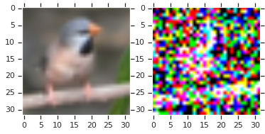
Interpreting pixel values as ‘emission probabilities’ results in unrealistic-looking samples - while it is an O.K. assumption for handwritten digits and sprites, it doesn't work for larger-scale, natural images. Papers that do use Bernoulli decoders will often showcase the emission probabilities (e.g. in a reconstruction or imputation task) rather than actual samples.

Pixel Values as Categorical Distributions

Larger color datasets (SVHN, CIFAR10, CelebA, ImageNet) are encoded in 8-bit RGB color (each channel is a uint8 integer that ranges in value from 0 to 255, inclusive).

Instead of interpreting their pixel values as Bernoulli emission probabilities, we can attempt to model the distribution over actual uint8 pixel values encoded in the image. One of the simplest choices is a 256-way categorical distribution.

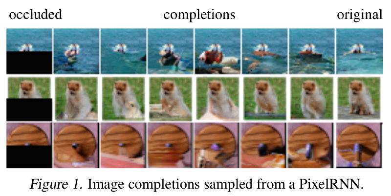Sampling from categorical distributions allows the generative model to sample images rather than emission probabilities.

For color images, it is common to report cross entropies of individual pixels in log base 2, instead of log base e. If a test set with 3072 pixels per image has average likelihood (nats) of $-H(p, q)$, the “bits-per-pixel” is just $-H(p, q)\div log (2)\div3072$.

This metric is motivated by average-likelihood-as-compression interpretation we discussed earlier: for a pixel that is typically encoded using 8 bits, we can devise a lossless entropy coding scheme using our generative model $p_\theta$ that can actually compress the entire dataset with an average bit length of 3 for representing each pixel.

At the time of this writing, the best generative model for Cifar10, Sparse Transformers, achieves a test likelihood of 2.80 bits per pixel. As a point of comparison, PNG and WebP -- widely used algorithms for lossless image compression -- achieve about 5.87 and 4.61 bits on Cifar10 images, respectively (PNG achieves 5.72 bpp if you don’t count the extra bytes like headers and CRC checksums).

This is quite exciting, because it suggests that machine learning can be used for better content-aware entropy-encoding schemes than existing compression schemes. Efficient lossless compression can be used to improve hashing algorithms, make your downloads faster, and improve your Zoom calls, and all of that technology is probably quite feasible today.

Stochastic De-Quantization for Continuous Density Models

If we optimize a continuous density model (such as a mixture of Gaussians) to maximize log-likelihood on discrete data, this can result in a degenerate solution where the model assigns the same density spike to each of the possible discrete values {0, ..., 255}. Even with an infinitely large dataset, the model can achieve arbitrarily high likelihoods by simply squeezing the spikes narrower and narrower.

To address this problem. it is quite common to de-quantize the data by adding noise to the integer pixel values. One such transformation is given by $y = x + u$, where $u$ is a sample from the random uniform $U(0,1)$. The first paper that I am aware of that motivates stochastic de-quantization for density modeling is Uria et al. 2013, and has since become common practice in Dinh et al., 2014, Salimans et al., 2017, and the works that built on top of these papers.

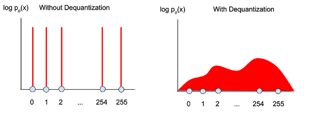Left: optimizing density models on discrete data can result in a degenerate solution where the model assigns a probability spike on a finite set of discrete values. Stochastic de-quantization is often applied so that we learn likelihood models on continuous data.

A discrete model assigns probability mass over an interval, while a continuous model assigns a density function. Let $P(x)$ and $p(x)$ represent the discrete probability masses and continuous densities of the true data distribution, and let $P_\theta(x)$ and $p_\theta(x)$ represent the same for the model density. We’ll derive below why optimizing the continuous likelihood model $p_\theta(y)$ over de-quantized data $y$ results in optimizing the lower-bound of the actual discrete probability model $P_\theta(x)$:

Integrating the density over a unit interval gives us the total mass implied by the density function:

$$ P_\theta(x) = \int_0^1 p_\theta(x+u) du $$

Our model likelihood objective is trained on de-quantized data sampled from the true data distribution:

$$ \mathbb{E}_{y \sim p}\left[ \log p_\theta(y) \right]$$

By definition of expectation:

$$ = \int p(y) \log p_\theta(y) dy $$

Expanding the integral,

$$ = \int dy p(y) \int dy \log p_\theta(x+du) $$
$$ = \mathbb{E}_{x \sim P} \int du \log p_\theta(x+du) $$


Via Jensen’s inequality (for the uniform variable u),

$$ \leq \mathbb{E}_{x \sim P} \log \int du p_\theta(x+du) $$
$$ = \mathbb{E}_{x \sim P} \log P_\theta(x) $$


A recent paper, Flow++, proposes using a learned de-quantization random variable to improve the tightness of the variational bound. The intuition here is that a single importance-sampled noise variate from $q(u|x)$ results in a lower-variance estimate of the integral $\int_0^1 p_\theta(x+u) du$ than a single sample from a uniform(0, 1) distribution. Because the de-quantization noise is different, one consequence of this work is that density models with different architectures and different quantization strategies cannot be compared in a controlled manner.

One way to compare Flow++ and uniformly de-quantized generative models fairly is to permit researchers to use whatever variational bound they like at training time, but standardize the evaluation of likelihood at evaluation time to be some tight multi-sample bound. The intuition here is that as we integrate over more samples, we get a better approximation of the true log-likelihood of the corresponding discrete model $P_\theta(x)$.

For instance, we could report the multi-sample bound from a fixed U(0, 1) de-quantization distribution, as commonly done in VAE literature with multi-sample IWAE bounds. A discussion of VAEs and IWAE bounds are out of the scope of this tutorial, and will be covered in the future.

Side Note: Data Preprocessing for Normalizing Flows

Normalizing Flows are a family of generative models that “transform” a base probability distribution into a more complicated probability distribution.





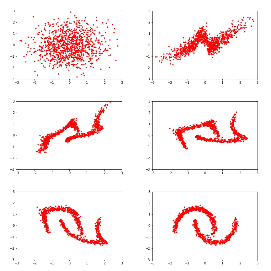
Normalizing Flows learn transformations that have tractable inverses and Jacobian determinants. Being able to compute these two quantities efficiently allow us to calculate the transformed distribution’s log-density, using the change-in-variables rule:


$$ \log p(y) = \log p(x) - \log |det J(f)(x)| $$


The vast majority of Normalizing Flows operate over continuous density functions (thus requiring the volume-tracking Jacobian determinant term), though there is some recent research on “discrete flows” that learn to transform probability mass functions rather than transforming density (Tran et al. 2019, Hoogeboom et al. 2019). We won’t be discussing these flows much in this blog post, but suffice it to say that they work by devising bijective discrete transformations of discrete base distributions.


In addition to the stochastic de-quantization mentioned earlier, there are a couple additional tricks employed when training normalizing flows for image data.

Empirically, re-scaling the data from the range [0, 256] to the unit interval [0, 1] prior to maximum likelihood estimation helps stabilize training, as neural network biases are usually centered around zero.

To prevent boundary issues where a sample from the base distribution could get mapped to a point outside of the re-scaled boundary (0, 1) by the flow, we can transform the re-scaled data to the range $-\infty, \infty$ via the logistic function (the inverse of the sigmoid function).


We can think of these re-scaling and logistic transforms as "preprocessing" flows at the beginning of the model, where just like any other bijector, we have to account for the change in volume induced by the transformation.

The important thing to realize here is that for evaluation purposes, pixel densities should always be computed in the continuous interval [0, 256], so that we can compare likelihoods from flows and autoregressive over the same data (up to the variational gap induced by the stochastic dequantization).

Here is a diagram showing a standard normalizing flow for RGB images, with the original discrete data on the left and the base density (can be a Gaussian, a logistic, or whatever your favorite tractable density is) on the right.





Generative model likelihoods typically reported in de-quantized space (green). Starting from Dinh et al. 2016, many flow-based models re-scale pixels to $[\lambda, 1-\lambda]$ and apply the logistic function (inverse sigmoid) to help with numerical stability on boundary conditions.

Discretized Logistic Mixture Likelihood

One drawback of modeling pixels with categorical distributions is that a categorical cross entropy loss cannot tell us that a pixel value of 127 is closer to 128 than it is to 0. For an observed pixel value $p$, the gradient of the categorical cross entropy is constant with respect to pixel intensity (since the loss treats the categories as un-ordered). Although the cross entropy gradient is non-zero, it is said to be “sparse” because it does not provide information on how close (in pixel intensity) we are to the target distribution. Ideally, we would like gradients to be larger in magnitude when the predicted intensity is far away from the observed value, and smaller when the model is close.

A more serious problem with modeling pixels as categorical distributions is that if we choose to represent more than 256 categories, we’d be in trouble. For example, we might want to model the R, G, and B pixels jointly (256^3 categories!) or model higher-precision pixel encodings than uint8 for HDR images. We’d quickly run out of memory attempting to store the projection matrices needed to map neural net activations to logits for that many categories.

Two concurrent papers, Inverse Autoregressive Flow and PixelCNN++, solve these problems by introducing a probability distribution for modeling RGB pixels as ordinal data, for which gradient information from the cross entropy loss can push pixels in the right direction while still preserving a discrete probability model.

We can model continuous pixel probability densities via a mixture of logistics, which is a continuous distribution. To recover probability mass for discrete pixel values, we can use the convenient property of the logistic distribution is that its CDF is the sigmoid function. By subtracting two sigmoids CDF(x+0.5) - CDF(x-0.5), we can recover the total probability mass lying between two integer pixel values.





For example, the probability of a pixel having value=127 is modeled as the probability mass lying between 126.5 and 127.5 for a continuous mixture of logistic distributions. The probability model must also account for edge cases such that CDF(0-0.5) is 0 and CDF(255+0.5) is 1, as is required of probability distributions.

Representing pixels in this way also affords the luxury of being able to handle a lot more categories, which means that PixelCNN++ can model the R, G, and B pixel channels at once. The caveat here is that you must tune the number of mixture components adequately (on Cifar-10, 5 seems to be enough).

Analogous to how Tran et al. 2019 devise discrete flows on top of categorical distributions, Hoogeboom et al. 2019 devise discrete flows for ordinal data by using this discretized logistic mixture likelihood as the base distribution. This gets the best of both worlds: we get to use normalizing flows for tractable inverses and sampling, while avoiding to have to solve for a de-quantized likelihood objective (which may incur a variational lower bound penalty on the likelihood). Both are very exciting papers that I hope to write about more in the future!

Perplexity

Log-likelihood is also a common metric for evaluating generative models in the language modeling domain. A discrete alphabet without ordering makes Categorical distributions the most natural choice for density modeling.

One quirk of the natural language processing (NLP) field is that language model likelihoods are often evaluated in units of Perplexity, which is given by $2^H(p, q)$. The inverse of perplexity, $\log_2 2^-H(p, q)$, is nothing more than average log-likelihood $-H(p, q)$. Perplexity is an intuitive concept since inverse probability is just the "branching factor" of a random variable, or the weighted average number of choices a random variable has. The relationship between perplexity and log-likelihood is so straightforward that some papers (Image Transformer) actually use the word “perplexity” interchangeably with log-likelihoods.

Closing Thoughts

In this blog post we derived the relationship between maximizing average log-likelihood and compression. We also mentioned several modeling choices between discrete and continuous likelihood models for individual pixels.

There is a broader question of whether likelihood is even the right quantity to be measuring / optimizing. At NIPS 2016 (now known as the NeurIPS conference), I recall there being a pretty lively debate in the generative modeling workshop where people were debating whether optimizing tractable-likelihood models was even a good idea.

It turns out that optimizing and evaluating against likelihood was a good idea after all, because since then researchers have figured out how to build and scale up much more flexible likelihood models while keeping them computationally tractable. Models like Glow, GPT-2, WaveNet, and Image Transformer are trained with likelihood and can generate image, audio and text samples with stunning quality. On the other hand, one might argue that at the end of the day, generative modeling needs to be coupled to performance on an actual task, such as classification accuracy when the model is fine-tuned on a labeled dataset. My colleague Niki Parmar says the following about images vs text likelihood models:

On text, there is generally a pattern where better likelihood leads to better performance on downstream tasks like GLUE. On images, I've heard from other practitioners that pixel prediction doesn't work as a pre-training task for downstream tasks like image classification. It could be because pixels don't mean much in terms of representations as compared to word-pieces or words in text. It's an open question but I find it fascinating that representation learning in images is quite different, almost difficult to establish and measure.

In a future blog post, I’ll build on top of this tutorial and discuss the evaluation of generative models that optimize variational lower bounds on log-likelihood (e.g. Variational Autoencoders, importance-weighted autoencoders).

Further Reading

• Twitter Thread discussing alternative metrics to the commonly reported log-likelihood and IWAE bounds.
• If you’re curious about what the compression ratios are for common lossless image compression algorithms, check out this script and paper.
• See the PixelRNN paper and this Reddit thread for further discussion on why categorical classification is preferable to continuous density modeling.
• Proper Local Scoring Rules - Thanks to Ferenc Huszár for pointing this paper out to me.
• A Note on the Evaluation of Generative Models - A terrific paper by Theis et al. that is a must-read for anyone getting started in the field of generative modeling.
• On the Quantitative Analysis of Decoder-based Generative Models
• Tutorial and Derivation of Perplexity, and this Stack Exchange question on Perplexity. Being unfamiliar with NLP myself, these links were super helpful for learning about the topic.
• The generative modeling community is fairly consistent about reporting MNIST in nats and color images in bits-per-dim, though some papers report MNIST likelihoods in bits/dim and others will report CIFAR10 in nats.
• This paper by Ranganath et al. proposes a general framework for thinking about variational inference (e.g. VAEs) by moving away from the standard KL divergence objective. One first imagines the desiderata they’d like to see in their divergence measure (e.g. sampling, preventing mode collapse), and then the paper proposes a method to recover a variational objective for the desired divergence. Thanks to Dustin Tran for pointing this one out to me. 

Acknowledgements

Many thanks to Dustin Tran, Niki Parmar, and Vincent Vanhoucke for reviewing drafts of this blog post. As always, thank you for reading!

Lessons from AI Research Projects: The First 3 Years

Translations: 中文

I've been at Google Brain robotics (now referred to as Robotics @ Google) for nearly 3 years. It's helpful to reflect, from time to time, on the scientific, engineering and personal productivity takeaways gleaned from working on large research projects. Every researcher's unique experiences and experimentation can potentially become their personal competitive edge for thinking about new problems in unique ways. Here are mine (so far).

These are ordered chronologically (earliest work first), so that the reader can see how my past experiences shape my current biases and beliefs (orange = first author).

Categorical Reparameterization with Gumbel-Softmax

• The importance of a work environment that encourages serendipitous discovery and 20% time (the inspiration for Gumbel-Softmax came to me in a water cooler conversation I was having with Shane Gu).
• Research on very basic techniques (e.g. generative modeling) can have a huge impact through various downstream applications.
• The simplest method to implement is the one that gets cited the most.

End-to-End Learning of Semantic Grasping

• The notion of a "class label" is meaningless, and is the wrong way to tackle goal-conditioned grasping.
• ML can help robotics, but robotics can also help ML (i.e. retroactive labeling via present poses).
• The importance of moving fast, investing in visualization and analysis tools (e.g. notebooks) that do not require a robot.

Time Contrastive Networks

• All you need is high-quality data and a contrastive loss. Pierre Sermanet is fond of saying, tongue-in-cheek, that these two things will get us to AGI.
• Dream big.

Deep Reinforcement Learning for Vision-Based Robotic Grasping

• The importance of a fast prototyping environment and quick experiment turnaround times.
• Q-Learning works and scales pretty well.

QT-Opt: Scalable Deep Reinforcement Learning for Vision-Based Robotic Manipulation

• Most people don’t really care how QT-Opt is trained; they are excited about what a trained QT-Opt system can do.
• All you need is scale, compute, and data.

Grasp2Vec: Learning Object Representations from Self-Supervised Grasping

• Magical things can happen if you focus on innovations in better-structured data, instead of better algorithms (all you need is high-quality data and a contrastive loss).
• The notion of a class label is meaningless.
• Good reward functions are a very nice piece of "Software 2.0" infrastructure: modular functionality, quick to verify for correctness, and does not impose strong assumptions on upstream or downstream computations (in contrast to RL algorithms).
• More on Twitter.

Generative Ensembles for Robust Anomaly Detection

• Thinking deeply about the nature of the OoD problem and different types of uncertainty. 
• The OoD problem is ill-posed, but still useful for practical applications.
• OoD and generalization are two sides of the same coin.
• I spent a 10 days in Jeju mentoring DL camp students. Every day I woke up, ate 3 meals in the same cafeteria downstairs, had no meetings, and thought really hard about the research problem. This monastic working environment was tremendously useful for my creative "flow".

Watch, Try, Learn: Meta-Learning from Demonstrations and Rewards

• Optimal control theory says that we need RL to make robots work, but you can get surprisingly far with the original Deep Learning recipe: supervised learning + lots of data + architecture tuning.
• Meta-Learning is all about pushing the burden of learning into the prior.
• Generative modeling (e.g. principled approaches to density estimation, being able to fit multi-modal distributions) is important for scaling up robotics.
• More on Twitter.

General Lessons from Deep RL + Robotics

• I am increasingly of the opinion that the biggest wins in making an ML system work come from high-quality data. Many researchers in sub-fields of ML do not prioritize the choice of data when looking for ways to improve on benchmarks. Deep RL on real robots is a great way to do ML research, because the researcher is forced to gather their own dataset and contend with how data biases generalization outcomes.
• Robotics is full-stack ML (gathering and serializing custom data, building a custom data pipeline, training and evaluation binaries, inference on a real robotic system), which increases iteration times & decreases opportunities for spontaneous creativity and discovery. Robotics projects tend to take ~1 FTE year to finish, while most DL papers can be completed in 2-3 months. One of the most important things to me right now is figuring out how we can achieve the same iteration speeds in robotics as achieved in other deep learning domains.
• Best software engineering practices for de-risking Deep RL engineering are in their early days. How to keep a full-stack dev environment flexible and fast to iterate on (scientific, creative risk) while keeping technical debt from bubbling over (execution risk)? My colleagues and I designed Tensor2Robot to solve a lot of our large-scale ML + robotics problems, but this is just the beginning.

The scope of this post is limited to my own research projects. Of course, there are papers that I didn't work on and inspire my views tremendously. I'll mention those in a follow-up blog post.

Fun with Snapchat's Gender Swapping Filter

Snapchat's new gender-bending filter is a source of endless fun and laughs at parties. The results are very pleasing to look at. As someone who is used to working with machine learning algorithms, it's almost magical how robust this feature is.

I was so duly impressed that I signed up for Snapchat and fiddled around with it this morning to try and figure out what's going on under the hood and how I might break it.

N.B, this is not a serious exercise in reverse-engineering Snapchat's IPA file or studying how other apps engineer similar features; it's just some basic hypothesis testing into when it works and when it doesn't, plus a little narcissistic bathroom selfie fun.


Initial Observations

The center picture is a standard bathroom selfie. To the left is the "male" filter, and on the right the "female" filter.

The first thing most users probably notice is that the app works in real time, works with a few different face angles, and does not require an internet connection to run. Hair behaves very naturally when wearing a beanie.

Here's a rotating profile shot. The app seems to detect whether the face is pointing in a permissible orientation, and only if that boolean is satisfied does the filter get applied.

Gender swap works in a variety of lighting conditions, though the hair does not seem to cast shadows.

Damn! I look cute.

Here was an example that I thought was really cool - the hair captures the directional key lighting.

Occlusion Tests

Ok, it works pretty well. Can we get it to fail? The app detects when the face is in the wrong pose, but what if there are things occluding the face? Do those occluding objects get "transformed" too?

The answer is yes. Below is a test where I slide an object across my face. The app works when half the face is occluded, but it seems like if too much of the face is blocked, the "should I face swap" bit is set to False.

Here's vertical occlusion, where the bit seems to depend on "what percentage of the face real estate is occluded" rather than what important semantic features (e.g. eyes, lips) are occluded. Right before the app decides that the "should I face swap" should switch to "False", you can see the blurring of the white bottle. Also, my hair turns blonde as I center the bottle in view.

Very interesting. This suggests to me that there definitely some machine learning going on here, and it's picking up on some statistical artifact of the data it was trained on. Do blondes tend to make more makeup tutorials or something?

I partially covered my face in a black charcoal masque, and things seemed pretty stable. The female filter does lighten the masque a bit. It's pretty easy to tell from this GIF that the "face swap" feature is confined to a rectangular region that tracks the head (note the sharp cutoff of the hair as it gets to my shoulders).

The filter stops working once I cover the rest of my face in the masque. Interestingly enough, the ovoid regions of my uncovered skin seem to be detected as faces, and the app proceeds to perform the style transform on that region. You can see the head and face templates flickering in and out like some kind of Junji Ito horror story.

Peeling off the masque is surprisingly stable.

Hair Layer

I was most impressed by the realism of the hair, so I wanted to figure out whether there were any hair mesh models used for dynamic lighting, or whether it was all machine-learning based.

The hair seems to be rendered as the topmost layer (like a Photoshop layer), but unlike your basic puppy ear/tongue filter, this hair layer has an alpha channel that is partially transparent. If you look closely there is also a clear segmentation mask for the hair that allows the face to show through. Snapchat is probably doing head tracking to figure out where the head is, computing the 2D alpha mask for the hair.


How does it work? A guess

At first glance, my mind jumped to some sort of CycleGAN architecture that maps the distribution of male faces to female faces, and vice versa. The dataset would be the billions of selfies Snap has, er, not deleted in the last 8 years.

This does raise a lot of questions though:

• Are they training truly unpaired image translation? That would be incredibly impressive, given that CycleGAN is bonkers and shouldn't even work in the first place. I would bet they have an unpaired alignment objective that is regularized by a limited dataset of ground-truth pairs, such as pairs of images of male/female siblings, or even a hand-designed gender transform that acts as data augmentation (e.g. making the jawline rounder can be done without machine learning). 
• The hair and face transforms seem to be synthesized independently, given that they occupy different layers (or perhaps synthesized together and separated into different layers right before rendering). This is also the first instance I've seen of GANs being used to render the alpha channel. I am a bit dubious of whether the hair is even generated by a GAN at all. One one hand, there is clearly some smooth function that switches out highlights and hair colors as a function of the positioning of an occluding object, suggesting that colors are probably learned partially from data. On the other hand, the hair is so stable that I have a hard time believing it is synthesized completely with a GAN generator. I have seen a few examples of other East Asian male face swaps with similar hairdos, suggesting that maybe there is a large-ish template library of haridos (that is refined with some ML model).
• How do Snap's ML engineers know whether a CycleGAN has converged for such an enormous dataset?
• How do they get these neural nets to run with such limited compute budgets? What sorts of image resolutions are they generating on the fly?

• If it indeed is a CycleGAN, then applying the male filter to a female-filtered image of me should recover the original image, right? 

• The image is mostly scale invariant, but as we zoom in pretty close, the face does resemble mine more. I would guess that there is a preprocessing step that crops and resizes the canonical face image prior to feeding it to a neural net.
• There are also probably other subroutines in the filter like jaw resizing that don't use a CycleGAN, but whose addition would cause the M2F and F2M filters to no longer be exact inverses of each other.

Implications of Technology

I have a friend who does drag. It's a lot of work! I'm excited for technology like this, because it will make it easier for makeup artists, cosplayers, and drag artists to experiment with new ideas and identities cheaply and quickly.

Technology such as face and voice changing enables a wider gap between public Internet personas and the real people managing those characters. This isn't necessarily a bad thing: if you are born a man but are passionate about being a cute anime girl on the internet, who are we to judge? Will gender fluidity & drag culture will become more normalized in society as our daily social media normalize gender-bending?

The future is quite exciting.

What I Cannot Control, I Do not Understand

Xiaoyi Yin has graciously translated this blog post to 中文.

I often hear the remark around the proverbial AI watering hole that there are no examples of reinforcement learning (RL) deployed in commercial settings that couldn’t be replaced by simpler algorithms.

This is somewhat true. If one takes RL to mean “neural networks trained with DQN / PPO / Soft-Actor Critic etc.”, then indeed, there are no commercial products (yet!) whose success relies on Deep RL algorithmic breakthroughs in the last 5 years [1].

However, if one interprets “reinforcement learning” to mean the notion of “learning from repeated trial and error”, then commercial applications abound, especially in pharmaceuticals, finance, TV show recommendations, and other endeavors based on scientific experimentation and intervention.

I’ll explain in this post how Reinforcement Learning is a general approach to solving the Causal Inference problem, the desiderata of nearly all machine learning systems. In this sense, many high-impact problems are already tackled using ideas from RL, but under different terminology and engineering processes.

Doctor, Won’t You Help Me Live Longer

Let’s suppose you are a doctor tasked with helping your patients live longer. You know a thing or two about data science, so you fit a model on a lot of patient records to predict life expectancy, and make a shocking finding: people who drink red wine every day have a 90% likelihood of living over 80 years, compared to the base probability of 50% for non drinkers.

In the parlance of causal inference, you’ve found the following observational distribution:

p(patient lives > 80 yrs | patient drinks red wine daily) = .9

Furthermore, your model has high accuracy on holdout datasets, which increases your confidence that your model has discovered the secret to longevity. Elated, you start telling your patients to drink red wine daily. After all, as a doctor, it is insufficient to predict; we must also prescribe! And what’s not to like about living longer and drinking red wine on the daily?

Many decades later, you follow up on your patients and -- with great disappointment -- observe the following interventional distribution:

p(patient lives > 80 yrs | do(patient drinks red wine daily)) = .5

The life expectancy of patients on the red wine has not increased! What gives?

Finding the Causal Model

The core problem here lies in confounding variables. When we decided to prescribe red wine to patients based on the observational model, we made a strong hypothesis about the causality diagram:

The directed edges between these random variables here denote causality, which can also be thought of as "the arrow of time". Changing the value of the “Drinks Red Wine” variable ought to have an effect on “Live > 80 years”, but changing “Lives > 80 years” has no effect on drinking red wine.

If this causal diagram was correct, then our intervention should have increased the lifespan of patients. But the actual experiment does not support this, so we must reject this hypothetical causal model and reach for alternative hypotheses to explain the data. Perhaps there are one or more variables that cause a higher propensity of red wine drinking, AND living longer, thus correlating those variables together?

We make the educated guess that a confounding variable might be that wealthy people tend to simultaneously live longer and drink more wine. Combing through the data again, we find that P(drinks red wine | is wealthy) = 0.9 and P(lives > 80 | is wealthy) = 1.0. So our hypothesis now takes the form:

If our understanding of the world is correct, then do(is wealthy) should make people live > 80 years and drink more red wine. And indeed, we find that once we give patients $1M cash infusions to make them wealthy (by USA standards), they end up living longer and drinking red wine daily (this is a hypothetical result, fabricated for the sake of this blog post).

RL as Automated Causal Inference

ML models are increasingly used to drive decision making in recommender systems, self-driving cars, pharmaceutical R&D, and experimental physics. In many cases, we desire an outcome event $y$, for which we attempt to learn a model $p(y|x_1, .., x_N)$ and then choose inputs $x_1...x_N$ to maximize $p(y|x_1...x_N)$.

It should be quite obvious from the previous medical example that to avoid causality when building decision-making systems is to risk overfitting models that are not useful for prescribing intervention. Suppose we automated the causal model discovery process in the following manner:

1. Fit an observational model to the data p(y|x_1, x_2, … x_N)
2. Assume the observational model captures the causal model. Prescribe an intervention do(x_i) that maximizes p(y|x_1..N) and gather a new dataset where 50% of x_i has the intervention and 50% does not.
3. Fit an observational model to the new data p(y|x_i)
4. Repeat steps 1-3 until observational model matches intervention model: p(y|do(x_i)) = p(y|x_i)

To return to the red wine case study as a test case:

1. You would initially have p(live > 80 years | drink red wine daily) = .9. 
2. Upon gathering a new dataset, you would obtain p(live > 80 years | do(drink red wine daily)) = .5. Model is not converged, but at least your observational model no longer believes that drinking red wine explains living longer. Furthermore, it now pays attention to the right variable, that p(live > 80 years | is_wealthy) = 1.
3. The subsequent iteration of this procedure then finds that p(live > 80 years | do(is wealthy)) = 1, so we are done.

The act of gathering a randomized trial (the 50% split of intervention vs. non-intervention) and re-training a new observational model is one of the most powerful ways to do general causal inference, because it uses data from reality (which “knows” the true causal model) to stamp out incorrect hypotheses.

Repeatedly training observational models and suggesting interventions is what RL algorithms are all about, which is solving optimal control for sequential decision-making problems. Control is the operative word here - the true test of whether an agent understands its environment is whether it can solve it.

For ML models whose predictions are used to infer interventions (so as to manipulate some downstream random variable), I argue that the overfitting problem is nothing more than a causal inference problem. This also explains why RL tends to be much harder as a machine learning problem than supervised learning - not only are there fewer bits of supervision per observation, but the RL agent must also figure out the causal, interventionist distribution required to behave optimally.

One salient case of “overfitting” is in RL algorithms can theoretically be trained “offline” -- that is, learning entirely from off-policy data without gathering new data samples from the environment. However, without periodically gathering new experience from the environment, agents can overfit to finite-size datasets or dataset imbalances, and propose interventions that do not generalize past their offline data. The best way to check if an agent is “learning the right thing” is to deploy it in the world and verify its hypotheses under the interventionist distribution. Indeed, for our robotic grasping research at Google, we often find that fine-tuning with “online” experience improves performance substantially. This is equivalent to re-training an observational model on new data p(grasp success | do(optimal_action)).


Production "RL"

The A/B testing framework often used in production engineering is a manual version of the "automated causal inference" pipeline, where a random 50% of users (assumed to be identically distributed) are shown one intervention and the other 50% are shown the control.

This is the cornerstone of data-driven decision making, and is used widely at hedge funds, Netflix, StitchFix, Google, Walmart, and so on. Although this process has humans in the loop (specifically for proposing interventions and choosing the stopping criterion), there are many related nuances to these methodologies that also arise in RL literature like data non-stationarity, the difficulty of obtaining truly randomized experiments, and long-term credit assignment. I’m just starting to learn about causal inference myself, and hope that in the next few years there will be more cross-fertilization of ideas between the RL, Data Science, and Causal Inference research communities.

For a more technical introduction to Causal Inference, see this great blog series by Ferenc Huszar.

[1] A footnote on why I think RL hasn’t had much commercial deployment yet. Feel free to clue me in if there are indeed companies using RL in production that I don’t know about!

In order for a company to be justified in adopting RL technology, the problem at hand needs to be 1) commercially useful 2) feasible for current Deep RL algorithms 3) the marginal utility of optimal control must be worth the technical risks of Deep RL.

Let’s consider deep image understanding by comparison: 1) everything from surveillance to self-driving cars to FaceID is highly commercially interesting 2) current models are highly accurate and scale well to a variety of image datasets 3) the models generally work as expected and do not require great expertise to train and deploy.

As for RL, it doesn’t take a great imagination to realize that general RL algorithms would eventually enable robots to learn skills entirely on their own, or help companies make complex financial decisions like stock buybacks and hiring, or enable far richer NPC behavior in games. Unfortunately, these problem domains don’t meet criteria (2) - the technology simply isn’t ready and requires many more years of R&D.

For problems where RL is plausible, it is difficult to justify being the first user of a technology whose marginal utility to your problem of choice is unproven. Example problems might include datacenter cooling or air traffic control. Even for domains where RL has been shown clearly to work (e.g. low-dimensional control or pixel-level control), RL still requires a lot of research skill to build a working system.